Warning: package 'ggplot2' was built under R version 4.2.3
Warning: package 'tidyr' was built under R version 4.2.3
Warning: package 'readr' was built under R version 4.2.3
Warning: package 'dplyr' was built under R version 4.2.3
Warning: package 'stringr' was built under R version 4.2.3
── Attaching core tidyverse packages ──────────────────────── tidyverse 2.0.0 ──
✔ dplyr     1.1.4     ✔ readr     2.1.5
✔ forcats   1.0.0     ✔ stringr   1.5.1
✔ ggplot2   3.5.0     ✔ tibble    3.2.1
✔ lubridate 1.9.3     ✔ tidyr     1.3.1
✔ purrr     1.0.2
── Conflicts ────────────────────────────────────────── tidyverse_conflicts() ──
✖ dplyr::filter() masks stats::filter()
✖ dplyr::lag()    masks stats::lag()
ℹ Use the conflicted package (<http://conflicted.r-lib.org/>) to force all conflicts to become errors
library(schrute)# Create a table from this package just corresponding to the Dinner Party episode:dinner_party_table <- theoffice |> dplyr::filter(season ==4) |> dplyr::filter(episode ==13) |># Just select columns of interest: dplyr::select(index, character, text)
TidyText processing of script
It’s very common to access data where a single column contains a long string of text, so that you have a long string of text in each row that you have to process. For instance, with the dinner_party_table dataset constructed above, the text column contains long strings which we can see by printing out the first so many rows:
head(dinner_party_table)
# A tibble: 6 × 3
  index character text
  <int> <chr>     <chr>
1 16791 Stanley   This is ridiculous.
2 16792 Phyllis   Do you have any idea what time we'll get out of here?
3 16793 Michael   Nobody likes to work late, least of all me. Do you have plans…
4 16794 Jim       Nope I don't, remember when you told us not to make plans 'ca…
5 16795 Michael   Yes I remember. Mmm, this is B.S. This is B.S. Why are we her…
6 16796 Dwight    Thank you Michael.
A token is a meaningful unit of text, most often a word, that we are interested in using for further analysis, and tokenization is the process of splitting text into tokens.
We can create this tidy dataset from our dinner_party_table using the unnest_tokens() function to break the various lines into tokens (aka tokenization). We specify what the new column will be called, word, given the source of the text, which is text here:
# install.packages("tidytext")library(tidytext)
Warning: package 'tidytext' was built under R version 4.2.3
tidy_dinner_party_tokens <- dinner_party_table |>unnest_tokens(word, text)# View the first so many rows:head(tidy_dinner_party_tokens)
# A tibble: 6 × 3
  index character word
  <int> <chr>     <chr>
1 16791 Stanley   this
2 16791 Stanley   is
3 16791 Stanley   ridiculous
4 16792 Phyllis   do
5 16792 Phyllis   you
6 16792 Phyllis   have
Each row of tidy_dinner_party_tokens corresponds to a single word spoken by a character (see character column) in the show during a single line (as reflected by the index column). We can see that the other columns are still in the data, but the text column has essentially been broken up into many rows. By default, punctuation marks are removed and all of the text is converted to lower case (which was helpful given the many lines in this episode that are in all caps!).
Before we continue to explore this dataset, we will remove stop words and perform stemming. First, we load a table of stop words from the tidytext package and simply filter them out from our data:
# load stop words in the tidytext packagedata(stop_words)# Next we can use the filter function to remove all stop words:tidy_dinner_party_tokens <- tidy_dinner_party_tokens |>filter(!(word %in% stop_words$word))# Alternatively, we can do this with the anti_join function:# tidy_dinner_party_tokens <- tidy_dinner_party_tokens |># anti_join(stop_words)
Next, we will use the SnowballC package to perform stemming:
# install.packages("SnowballC")library(SnowballC)tidy_dinner_party_tokens <- tidy_dinner_party_tokens |># Create a new column stem with the wordStem function:mutate(stem =wordStem(word))# View the update:head(tidy_dinner_party_tokens)
# A tibble: 6 × 4
  index character word       stem
  <int> <chr>     <chr>      <chr>
1 16791 Stanley   ridiculous ridicul
2 16792 Phyllis   idea       idea
3 16792 Phyllis   time       time
4 16793 Michael   likes      like
5 16793 Michael   late       late
6 16793 Michael   plans      plan
Word clouds
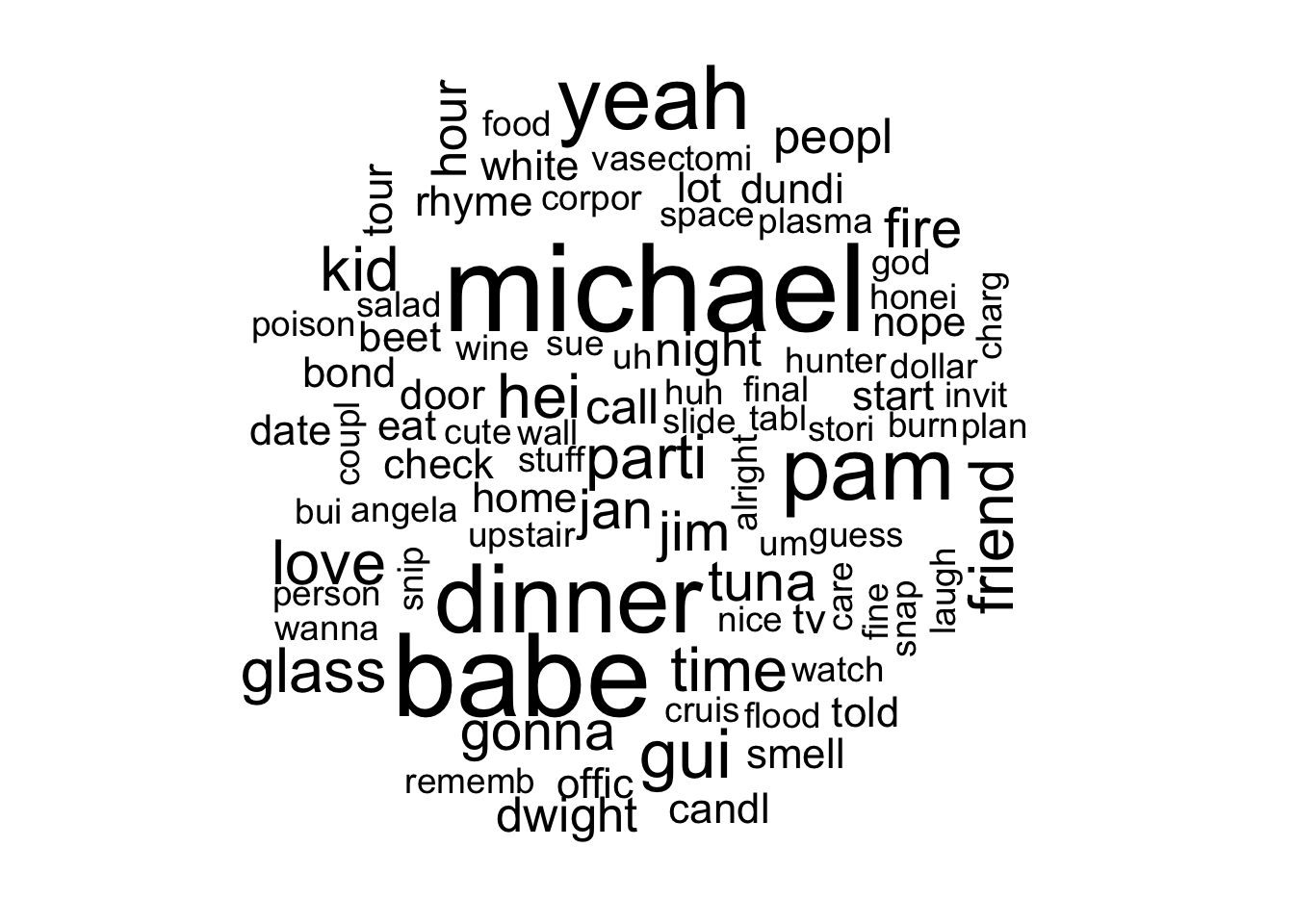
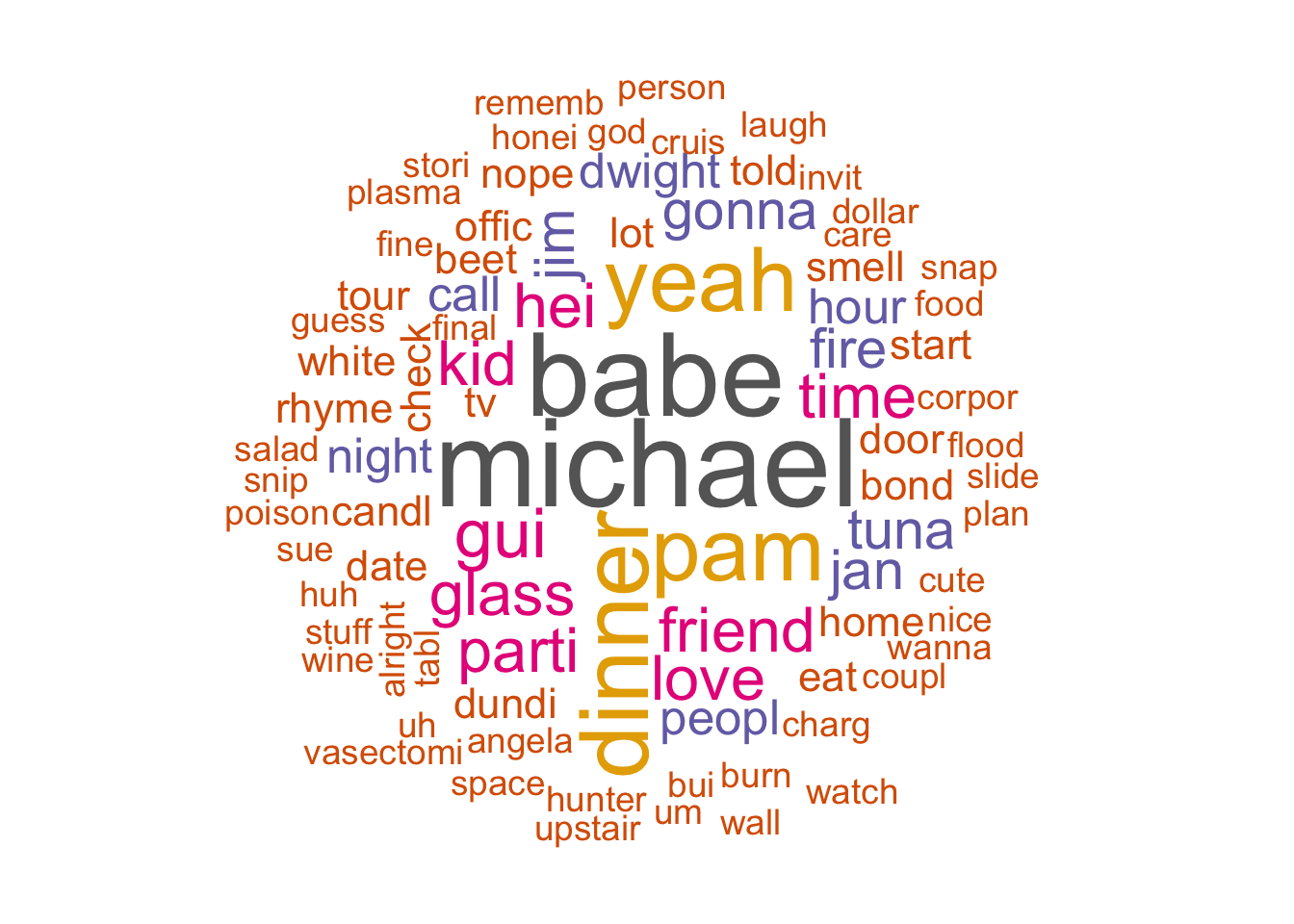
From this dataset, we technically have everything we need to construct the wider document-term (or term-document) matrices. But in the current format, we can take advantage of the tidyverse syntax we’re used to with group_by() and summarize() to compute quantities we’re interested in the ways we want. For instance, we can compute the frequency of each stem across all spoken lines and characters then create a word cloud by just grabbing the appropriate columns.
Word clouds are probably the most well-known way of visualizing text data. Word clouds show the most common words in a set of documents, with more common words being bigger in the word cloud. To make word clouds in R, you’ll need the wordcloud library. When you look at the help documentation for the wordcloud() function, you’ll see that there are two main arguments: words and freq, which correspond to the words in the documents and their frequencies, respectively.
# First create a dataset counting the number of each stem across the full scripttoken_summary <- tidy_dinner_party_tokens |>group_by(stem) |># Instead of summarize we can use the count functioncount() |>ungroup() # Now make a wordcloud :library(wordcloud)
There are a few things we can do to make the word cloud a bit prettier. First, it is more typical to place the biggest words in the center of the word cloud; this can be done by setting random.order = FALSE within wordcloud(). Furthermore, in the above word cloud we see that there are a bunch of tiny terms, and usually these are thrown out; you can control how many words are plotted on your word cloud by controlling max.words within wordcloud(). For example, we set max.words = 100, meaning the resulting word cloud displays the 100 most frequent words. We can also change the color palette; above you can see that loading the wordcloud library automatically loads the RColorBrewer library, and you can use functions like brewer.pal() like I do below to set the colors of the word cloud. There are lots of arguments within the wordcloud() function, so I encourage you to explore this function if you’re interested.
While could treat each spoken line as a separate document (index), instead we can focus on a collection of documents based on the characters speaking the lines (character). This corresponds to grouping by character instead of index. The following creates the token/stem count summary by character:
character_token_summary <- tidy_dinner_party_tokens |>group_by(character, stem) |># Instead of summarize we can use the count functioncount() |>ungroup() head(character_token_summary)
# A tibble: 6 × 3
  character stem       n
  <chr>     <chr>  <int>
1 All       cheer      1
2 Andy      anim       1
3 Andy      bet        1
4 Andy      capit      1
5 Andy      dinner     1
6 Andy      flower     2
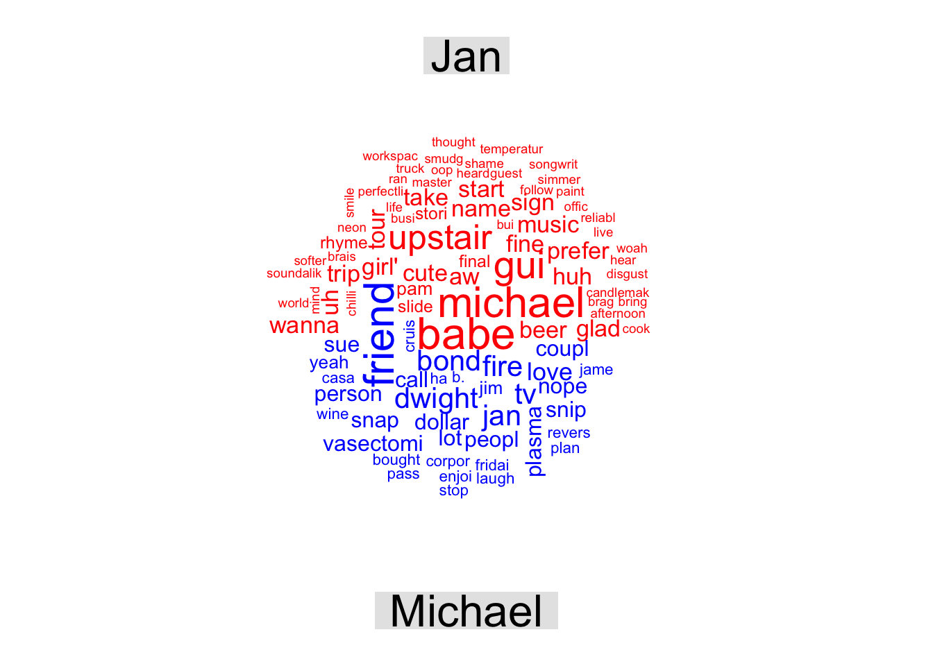
We’re now going to create a comparison word cloud to compare the frequencies of words between two characters in this episode: Michael and Jan. First, we create a table below that only contains the word counts for michael and jan:
Next, we can use the comparison.cloud() function to get a sense of which words are more unique to each character as explained in the Concept 2 material. However, we need to reshape the data in such a way that each row is a word and there are two columns, one for each character to reflect the number of times that word appears for each character. The labels for the words need to be stored in the row names of this matrix. Fortunately, this convoluted process is rather easy to perform using the reshape2 package and the acast function as demonstrated below:
library(reshape2)
Attaching package: 'reshape2'
The following object is masked from 'package:tidyr':

    smiths
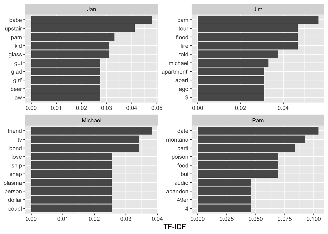
We can easily compute and join the TF-IDF values for each stem treating the different characters as documents with the bind_tf_idf() function. All this requires is three input columns referring to words, documents, and counts. TF-IDF will down-weigh words that occur frequently across all documents and will upweigh words that uniquely occur in certain documents. In our example, these are: stem, character, n:
# A tibble: 6 × 6
  character stem       n     tf   idf tf_idf
  <chr>     <chr>  <int>  <dbl> <dbl>  <dbl>
1 All       cheer      1 1      2.77  2.77
2 Andy      anim       1 0.0476 2.77  0.132
3 Andy      bet        1 0.0476 2.08  0.0990
4 Andy      capit      1 0.0476 2.77  0.132
5 Andy      dinner     1 0.0476 0.981 0.0467
6 Andy      flower     2 0.0952 2.77  0.264
Note that the tf column here refers to the term-frequency calculated as the number of times the character said that specific word/stem (by that character) divided by the total number of words/stems spoken by that character. The idf column refers to the inverse-document frequency column from lecture.
We can proceed to create a visual displaying the top 10 words/stems in terms of importance by TF-IDF for characters in the episode. For simplicity, we’ll just consider the four characters with the most lines in the episode based on the following:
    Michael         Jan         Jim         Pam      Dwight      Angela
         89          73          38          28          16          12
       Andy       Woman   Officer 1   Officer 2         All Hunter's CD
         10           5           3           2           1           1
     Michae     Officer     Phyllis     Stanley
          1           1           1           1
The following code chunk now displays the top 10 stems sorted by TF-IDF for Michael, Jan, Jim, and Pam. We use the reorder_within() function from the tidytext package to make sure the bars are sorted within the facets:
character_token_summary |># Just grab the four characters of interest:filter(character %in%c("Michael", "Jan", "Jim", "Pam")) |># Group by character and just use the top 10 based on tf_idf with slice_maxgroup_by(character) |>slice_max(tf_idf, n =10, with_ties =FALSE) |>ungroup() |>mutate(stem =reorder_within(stem, tf_idf, character)) |>ggplot(aes(y = tf_idf, # We use the fct_reorder to sort the bars within the facetsx = stem),fill ="darkblue", alpha =0.5) +geom_col() +coord_flip() +scale_x_reordered() +facet_wrap(~ character, ncol =2, scales ="free") +labs(y ="TF-IDF", x =NULL)
Sentiment Analysis
There are also techniques for measuring the overall “sentiment” of a document. These techniques are usually dictionary-based; for example, one can come up with a list of “positive” words and “negative” words (i.e., positive and negative dictionaries), and then count the number of positive and negative words that occur in a document. Thus, you can get an aggregate measure of how “positive” or “negative” a piece of text is. There are many different ways to define the “sentiment” of text (see the References and Resources section below); for this example, we’re just going to focus on “positive” versus “negative” text.
Again we’re going to focus on the episode’s script, and first, we’re going to process the data as we did before in the previous section. However, unlike the previous section, we are not going to remove stop words or perform stemming - for sentiment analysis, it’s important to keep individual words that may have certain types of sentiment.
Now: Which of these words are “positive” words and which of these words are “negative” words? There’s a function in the tidytext library called get_sentiments(). There are many different “sentiment dictionaries” available within this function, and we’re going to just focus on get_sentiments("bing"), which provides a bunch of words that are deemed either “positive” or “negative” in a binary fashion:
In what follows, we’re going to join the binary sentiment assignment to the tidy token table - and only keep the words with an assignment based on the inner_join() function:
# Label each word with a positive or negative sentiment# (if it has one)tidy_sentiment_tokens <- tidy_all_tokens |>inner_join(get_sentiments("bing"))# View the head of this:head(tidy_sentiment_tokens)
# A tibble: 6 × 4
  index character word       sentiment
  <int> <chr>     <chr>      <chr>
1 16791 Stanley   ridiculous negative
2 16793 Michael   likes      positive
3 16793 Michael   work       positive
4 16795 Michael   enough     positive
5 16795 Michael   enough     positive
6 16795 Michael   mad        negative
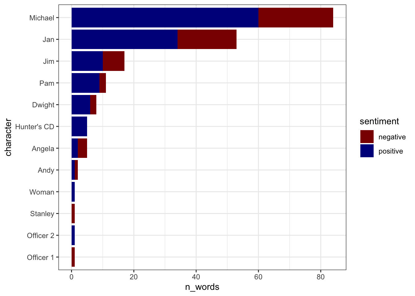
So now we can see how the characters vary in terms of “positive” or “negative” words. We can simply count up the total number of “positive” and “negative” words said by each character:
We can then display how the characters compare with stacked bar charts indicating how many positive and negative words were said by each character (ordering the characters by the total number of assigned words):
character_sentiment_summary |>group_by(character) |>mutate(total_assigned_words =sum(n_words)) |>ungroup() |># Reorder the characters by the total number of words:mutate(character =fct_reorder(character, total_assigned_words)) |># Display stacked barsggplot(aes(x = character, y = n_words, fill = sentiment)) +geom_bar(stat ="identity") +coord_flip() +scale_fill_manual(values =c("darkred", "darkblue")) +theme_bw()
From this, we can see the most characters seem to say more positive words than negative words (except for Angela…). But we can see how the proportions within characters appears to vary, e.g., Pam has a much higher proportion of positive words than Jim.
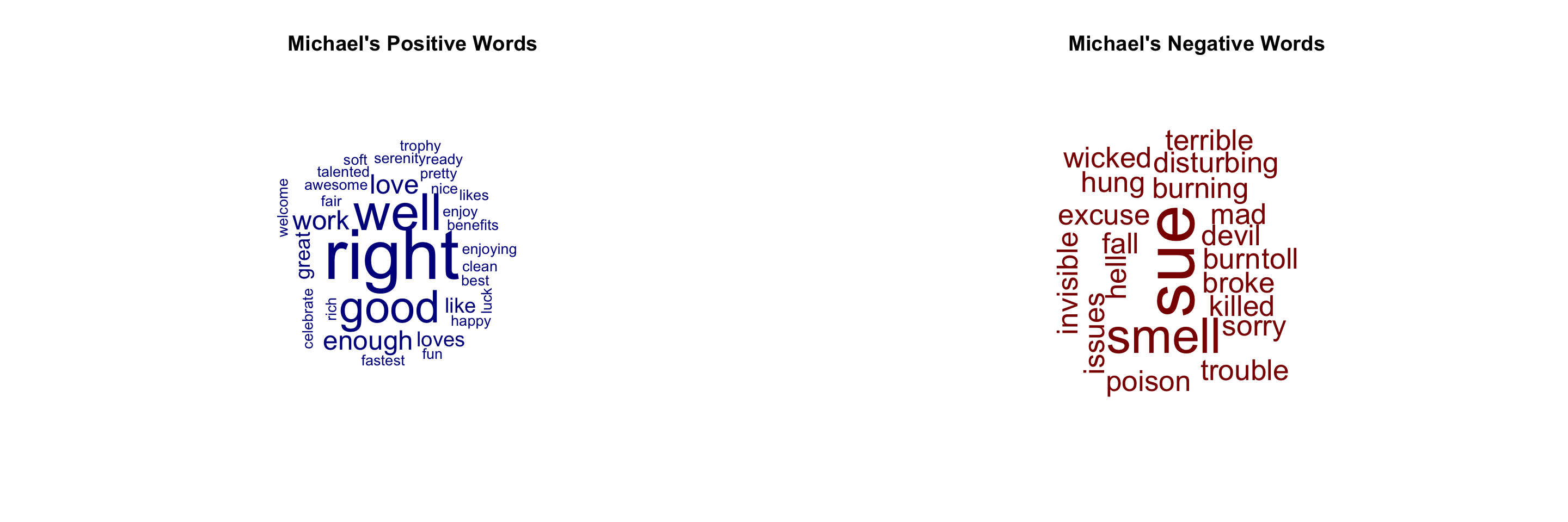
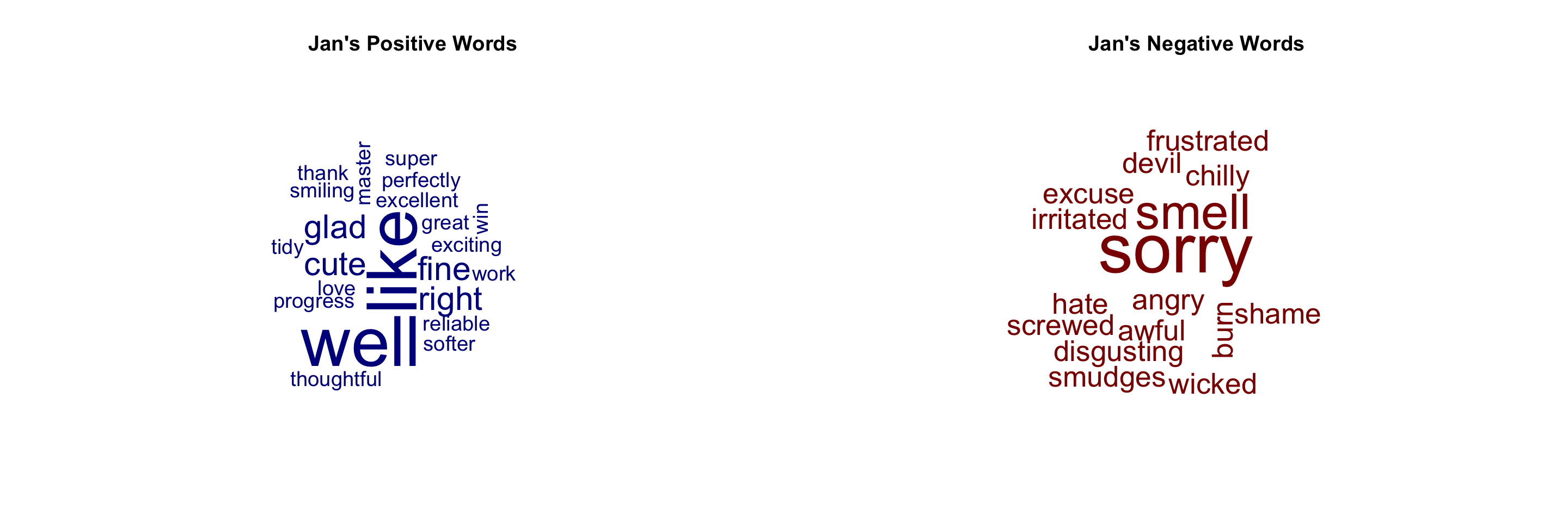
It’s also common to make word clouds of “positive” words and “negative” words, so that one can get an idea of the common words expressing “positive” or “negative” sentiment in a set of documents. Below, we separate words said by the two characters with the most dialogue in the episode, Michael and Jan, then separate out their positive and negative words to create word clouds.
# First for Michael, make the positive summary:michael_positive_summary <- tidy_sentiment_tokens |>filter(character =="Michael", sentiment =="positive") |>group_by(word) |>count()# Now Michael's negative summary:michael_negative_summary <- tidy_sentiment_tokens |>filter(character =="Michael", sentiment =="negative") |>group_by(word) |>count()# Now make the word clouds for these two tables:par(mfrow =c(1,2))# word cloud for Michael's positive wordswordcloud(words = michael_positive_summary$word,freq = michael_positive_summary$n,random.order =FALSE, color ="darkblue", min.freq =1)title(main ="Michael's Positive Words")# word cloud for Michael's negative wordswordcloud(words = michael_negative_summary$word,freq = michael_negative_summary$n,random.order =FALSE, color ="darkred", min.freq =1)title(main ="Michael's Negative Words")
# Next for Jan, make the positive summary:jan_positive_summary <- tidy_sentiment_tokens |>filter(character =="Jan", sentiment =="positive") |>group_by(word) |>count()# Now Jan's negative summary:jan_negative_summary <- tidy_sentiment_tokens |>filter(character =="Jan", sentiment =="negative") |>group_by(word) |>count()# Now make the word clouds for these two tables:par(mfrow =c(1,2))# word cloud for Jan's positive wordswordcloud(words = jan_positive_summary$word,freq = jan_positive_summary$n,random.order =FALSE, color ="darkblue", min.freq =1)title(main ="Jan's Positive Words")# word cloud for Jan's negative wordswordcloud(words = jan_negative_summary$word,freq = jan_negative_summary$n,random.order =FALSE, color ="darkred", min.freq =1)title(main ="Jan's Negative Words")