2D Quantitative Data
2024-09-11
Reminders, previously, and today…
Finished up discussion of 1D quantitative visualizations
Discussed impact of bins on histograms
Covered ECDFs and connection to KS-tests
Walked through density estimation and ways of visualizing conditional distributions
2D quantitative data
We’re working with two variables: \((X, Y) \in \mathbb{R}^2\) , i.e., dataset with \(n\) rows and 2 columns
Goals:
describing the relationships between two variables
describing the conditional distribution \(Y | X\) via regression analysis
describing the joint distribution \(X,Y\) via contours, heatmaps, etc.
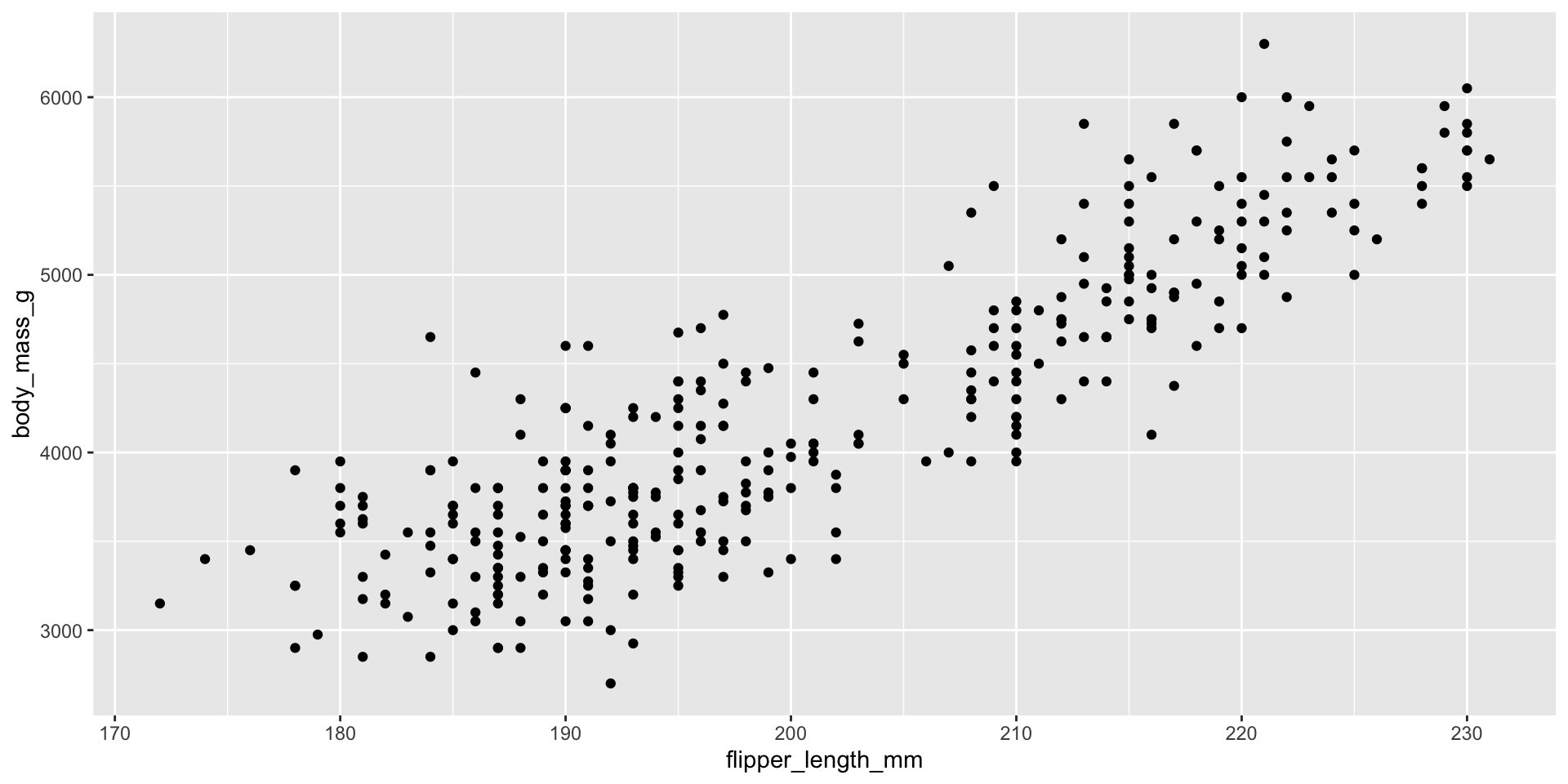
Making scatterplots with geom_point()
|> ggplot (aes (x = flipper_length_mm, y = body_mass_g)) + geom_point ()
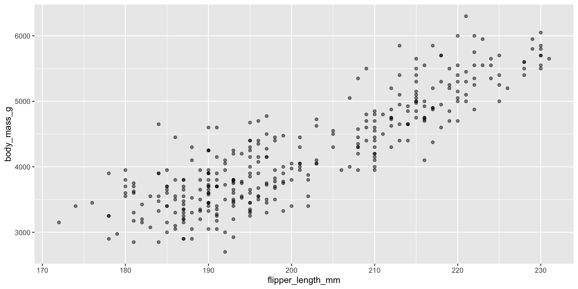
Making scatterplots: ALWAYS adjust the alpha
|> ggplot (aes (x = flipper_length_mm, y = body_mass_g)) + geom_point (alpha = 0.5 )
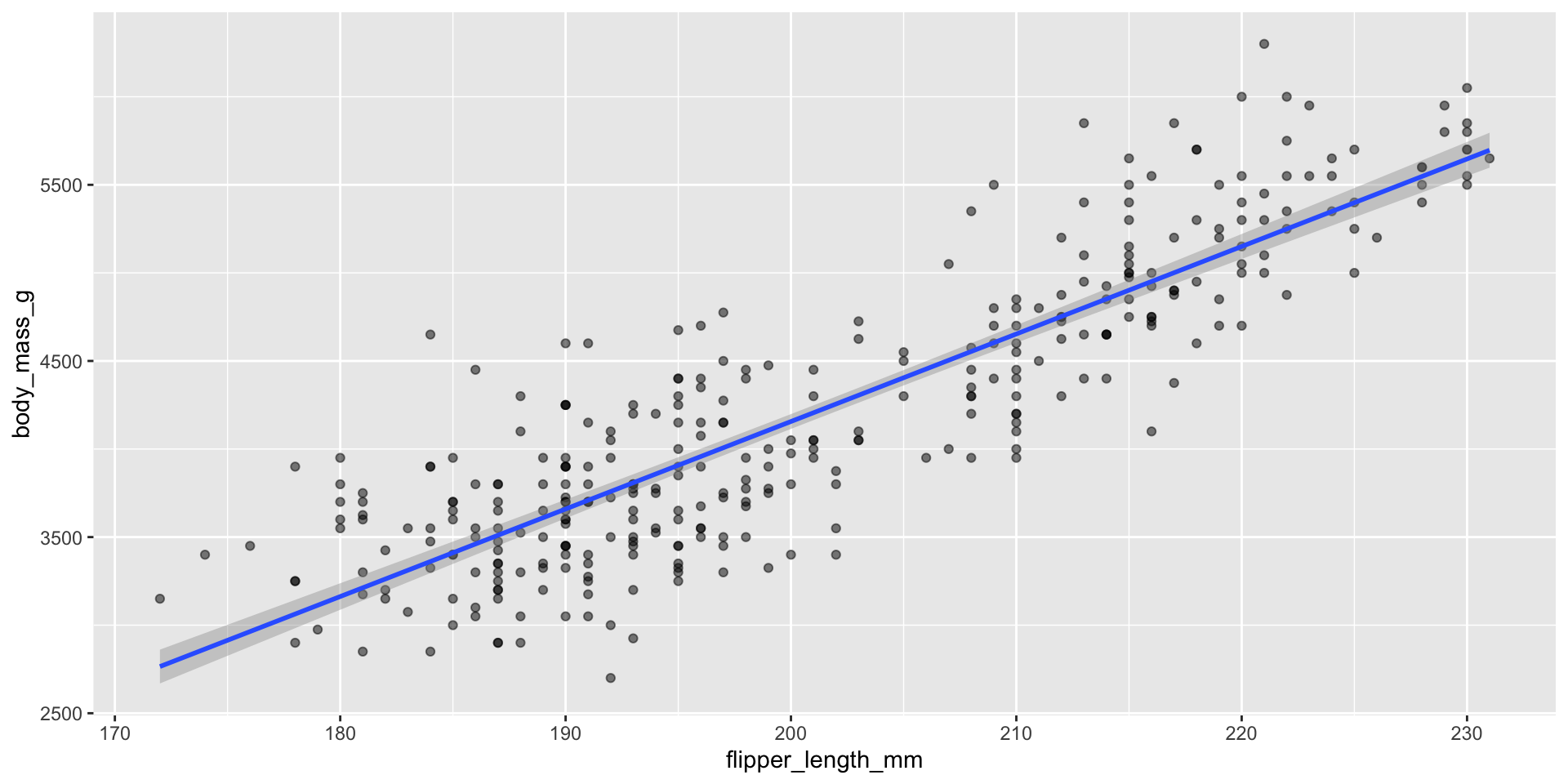
Displaying trend lines: linear regression
|> ggplot (aes (x = flipper_length_mm, y = body_mass_g)) + geom_point (alpha = 0.5 ) + geom_smooth (method = "lm" )
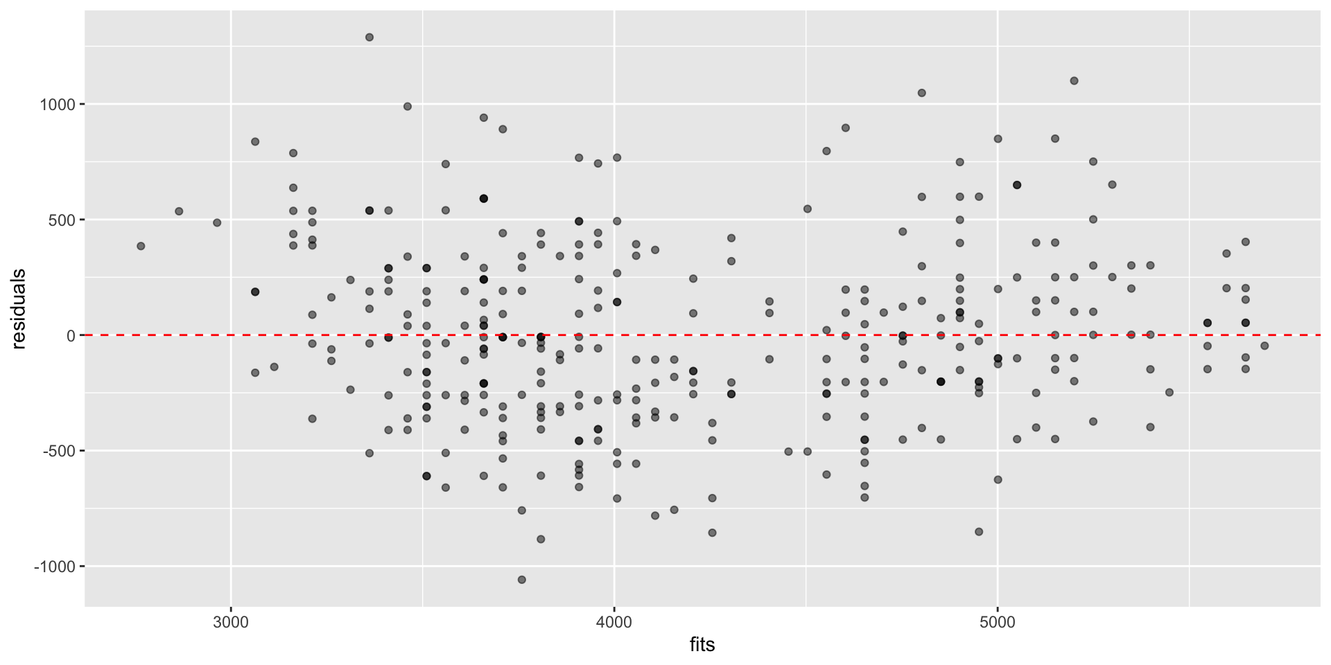
Assessing assumptions of linear regression
Linear regression assumes \(Y_i \overset{iid}{\sim} N(\beta_0 + \beta_1 X_i, \sigma^2)\)
If this is true, then \(Y_i - \hat{Y}_i \overset{iid}{\sim} N(0, \sigma^2)\)
Plot residuals against \(\hat{Y}_i\) , residuals vs fit plot
Used to assess linearity, any divergence from mean 0
Used to assess equal variance, i.e., if \(\sigma^2\) is homogenous across predictions/fits \(\hat{Y}_i\)
More difficult to assess the independence and fixed \(X\) assumptions
Make these assumptions based on subject-matter knowledge
Residual vs fit plots
<- lm (body_mass_g ~ flipper_length_mm, data = penguins)tibble (fits = fitted (lin_reg), residuals = residuals (lin_reg)) |> ggplot (aes (x = fits, y = residuals)) + geom_point (alpha = 0.5 ) + geom_hline (yintercept = 0 , linetype = "dashed" , color = "red" )
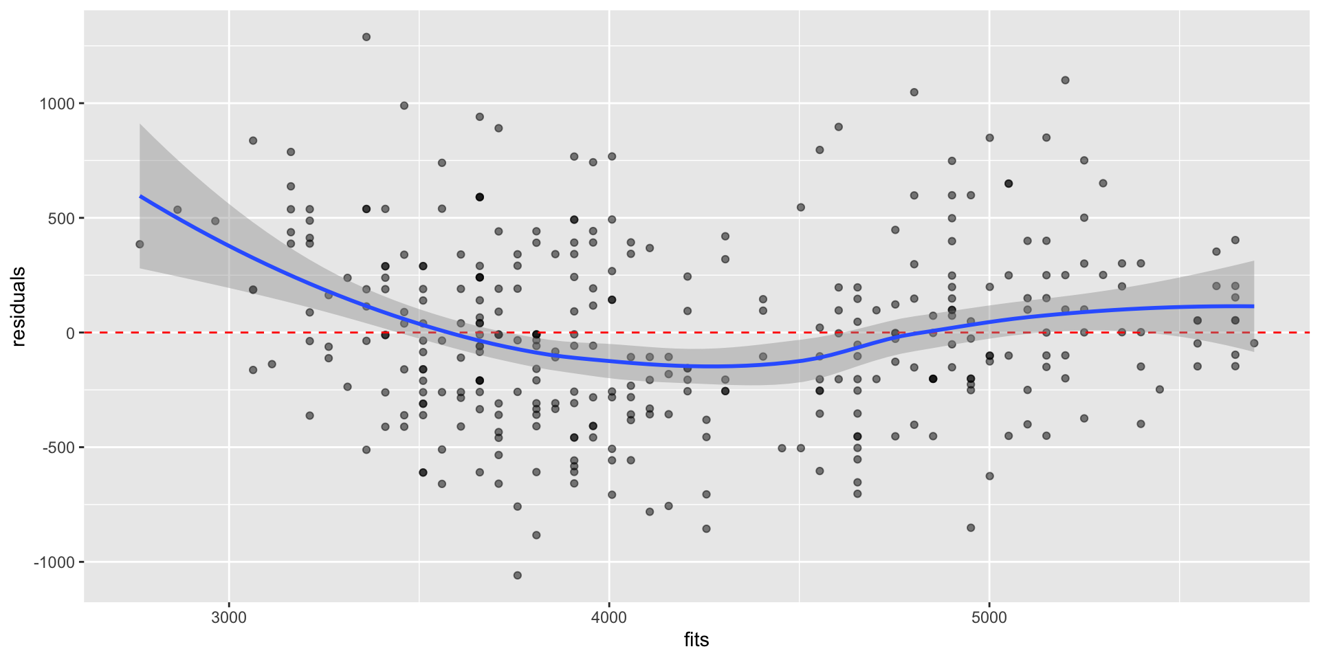
Residual vs fit plots
tibble (fits = fitted (lin_reg), residuals = residuals (lin_reg)) |> ggplot (aes (x = fits, y = residuals)) + geom_point (alpha = 0.5 ) + geom_hline (yintercept = 0 , linetype = "dashed" , color = "red" ) + geom_smooth ()
Local linear regression via LOESS
\(Y_i \overset{iid}{\sim} N(f(x), \sigma^2)\) , where \(f(x)\) is some unknown function
In local linear regression , we estimate \(f(X_i)\) :
\[\text{arg }\underset{\beta_0, \beta_1}{\text{min}} \sum_i^n w_i(x) \cdot \big(Y_i - \beta_0 - \beta_1 X_i \big)^2\]
geom_smooth() uses tri-cubic weighting:
\[w_i(d_i) = \begin{cases} (1 - |d_i|^3)^3, \text{ if } i \in \text{neighborhood of } x, \\
0 \text{ if } i \notin \text{neighborhood of } x \end{cases}\]
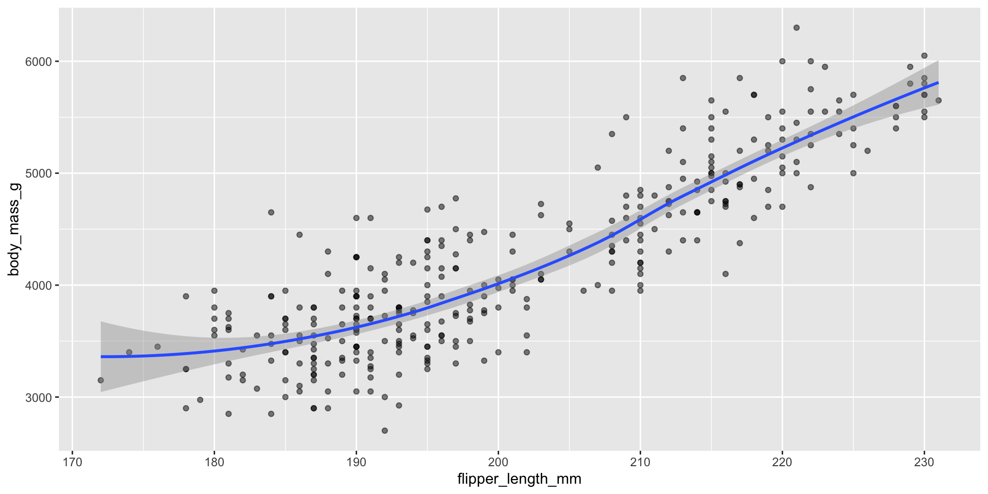
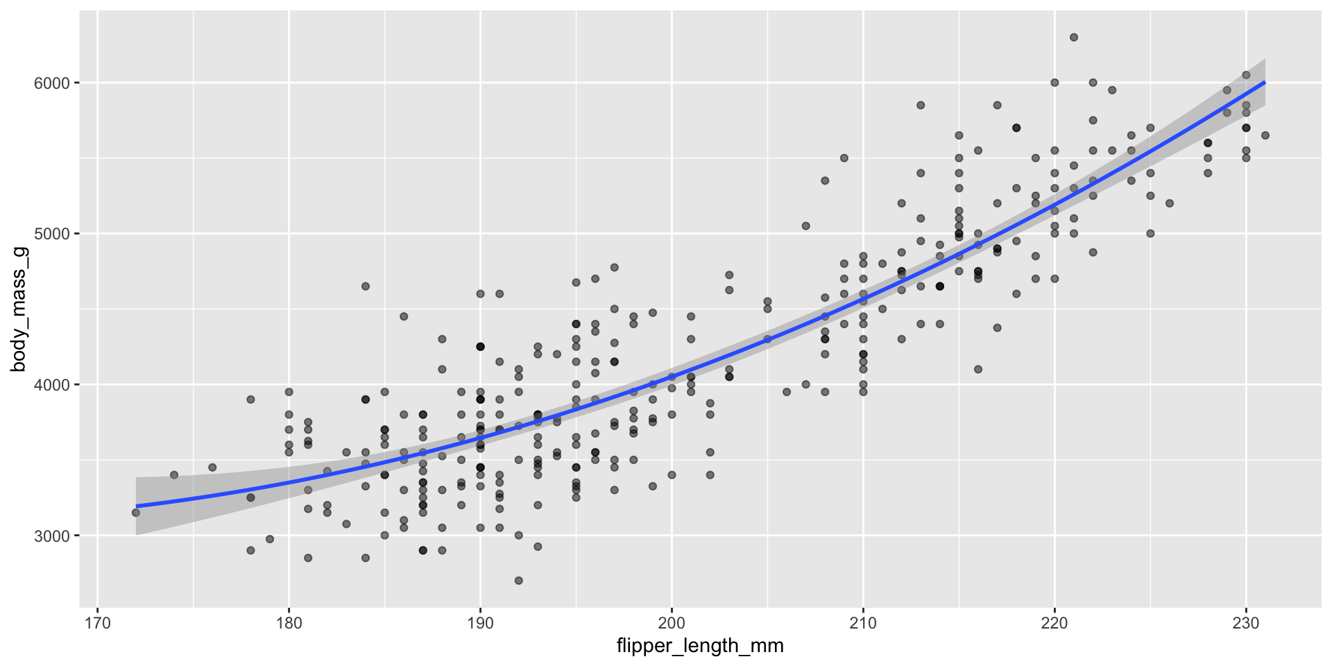
Displaying trend lines: LOESS
|> ggplot (aes (x = flipper_length_mm, y = body_mass_g)) + geom_point (alpha = 0.5 ) + geom_smooth ()
For \(n > 1000\) , mgcv::gam() is used with formula = y ~ s(x, bs = "cs") and method = "REML"
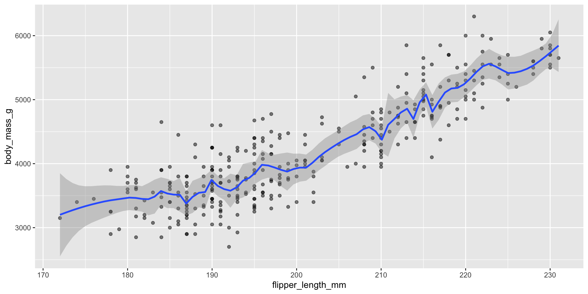
Displaying trend lines: LOESS
|> ggplot (aes (x = flipper_length_mm, y = body_mass_g)) + geom_point (alpha = 0.5 ) + geom_smooth (span = .1 )
What about focusing on the joint distribution?
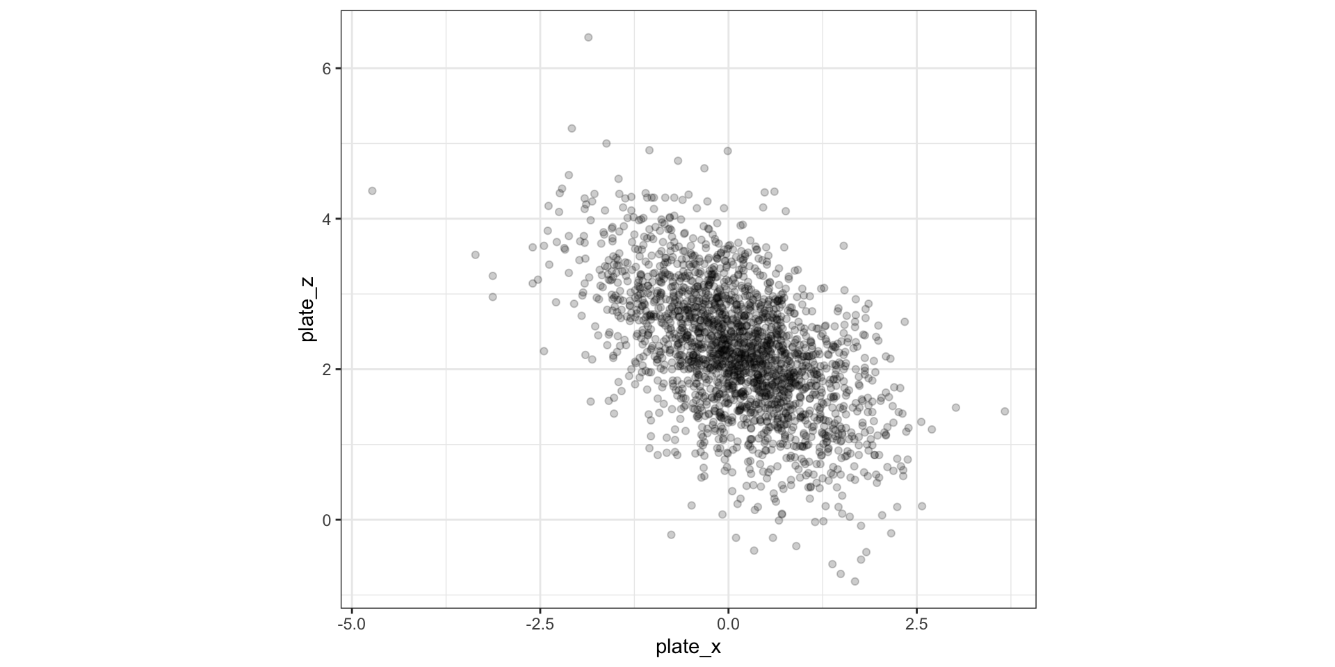
Example dataset of pitches thrown by baseball superstar Shohei Ohtani
|> ggplot (aes (x = plate_x, y = plate_z)) + geom_point (alpha = 0.2 ) + coord_fixed () + theme_bw ()
Going from 1D to 2D density estimation
In 1D: estimate density \(f(x)\) , assuming that \(f(x)\) is smooth :
\[
\hat{f}(x) = \frac{1}{n} \sum_{i=1}^n \frac{1}{h} K_h(x - x_i)
\]
In 2D: estimate joint density \(f(x_1, x_2)\)
\[\hat{f}(x_1, x_2) = \frac{1}{n} \sum_{i=1}^n \frac{1}{h_1h_2} K(\frac{x_1 - x_{i1}}{h_1}) K(\frac{x_2 - x_{i2}}{h_2})\]
In 1D there was one bandwidth, now we have two bandwidths
\(h_1\) : controls smoothness as \(X_1\) changes, holding \(X_2\) fixed\(h_2\) : controls smoothness as \(X_2\) changes, holding \(X_1\) fixed
Again Gaussian kernels are the most popular…
So how do we display densities for 2D data?
How to read contour plots?
Best known in topology: outlines (contours) denote levels of elevation
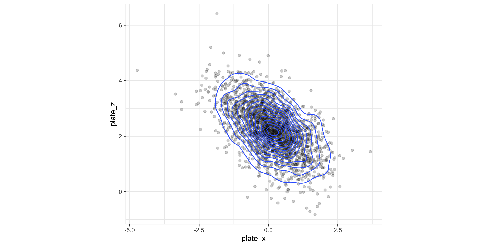
Display 2D contour plot
|> ggplot (aes (x = plate_x, y = plate_z)) + geom_point (alpha = 0.2 ) + geom_density2d () + coord_fixed () + theme_bw ()
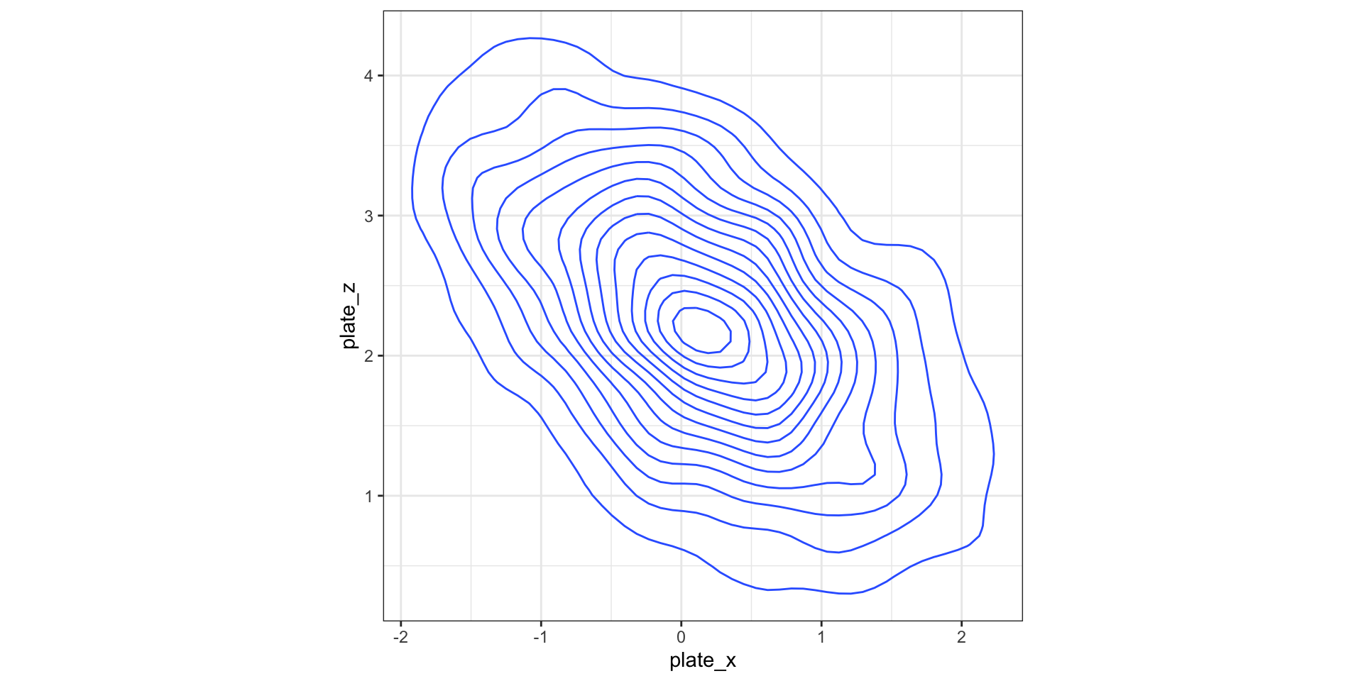
Display 2D contour plot
|> ggplot (aes (x = plate_x, y = plate_z)) + geom_density2d () + coord_fixed () + theme_bw ()
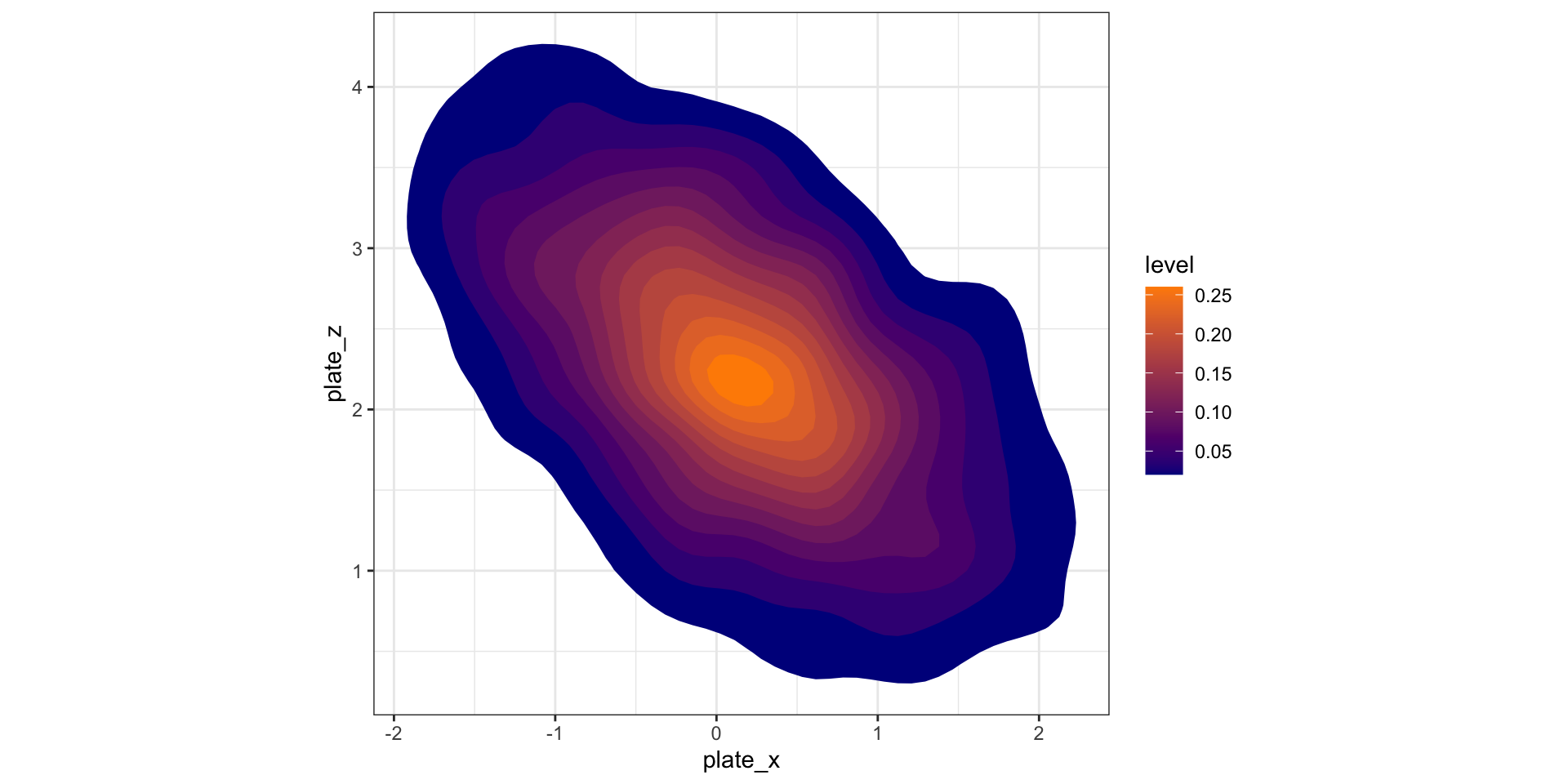
Display 2D contour plot
|> ggplot (aes (x = plate_x, y = plate_z)) + stat_density2d (aes (fill = after_stat (level)), geom = "polygon" ) + coord_fixed () + scale_fill_gradient (low = "darkblue" , high = "darkorange" ) + theme_bw ()
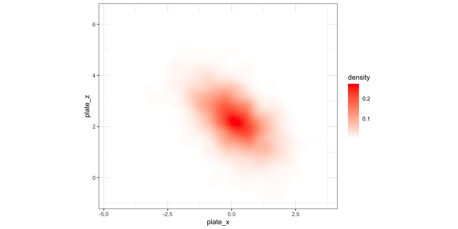
Visualizing grid heat maps
|> ggplot (aes (x = plate_x, y = plate_z)) + stat_density2d (aes (fill = after_stat (density)), geom = "tile" , contour = FALSE ) + coord_fixed () + scale_fill_gradient (low = "white" , high = "red" ) + theme_bw ()
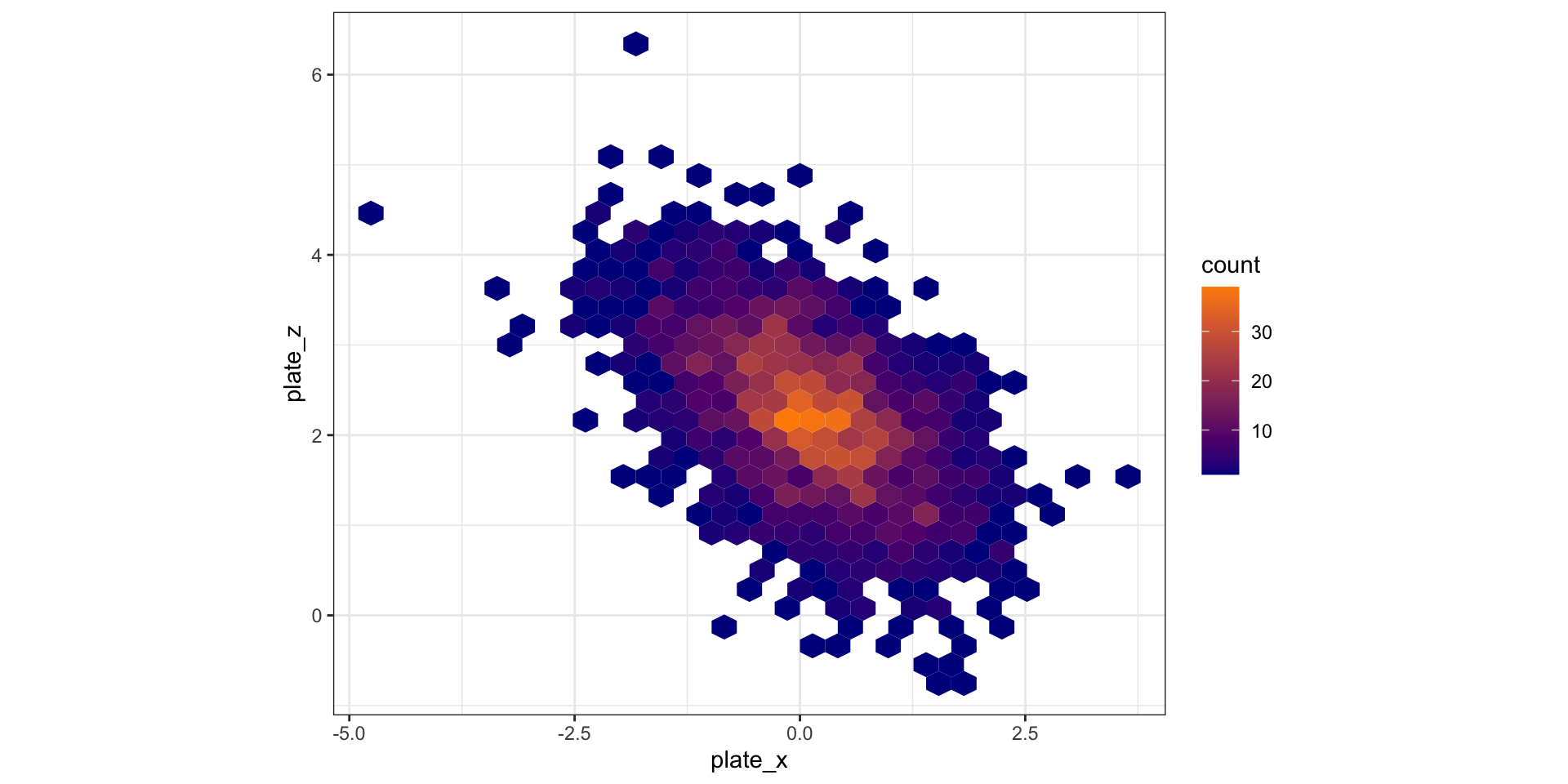
Alternative idea: hexagonal binning
|> ggplot (aes (x = plate_x, y = plate_z)) + geom_hex () + coord_fixed () + scale_fill_gradient (low = "darkblue" , high = "darkorange" ) + theme_bw ()
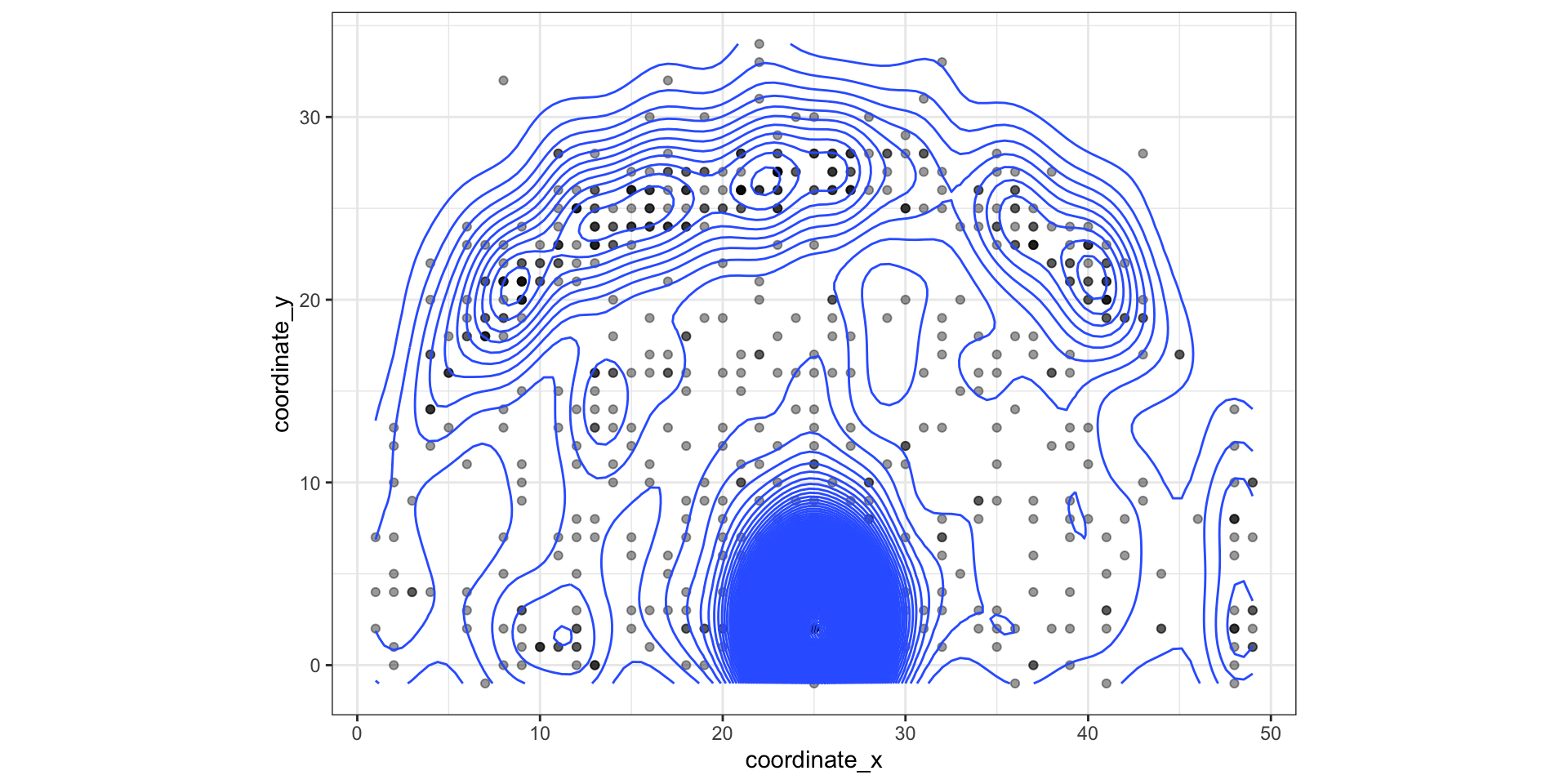
<- read_csv ("https://raw.githubusercontent.com/ryurko/DataViz-Class-Data/main/lebron_shots.csv" )|> ggplot (aes (x = coordinate_x, y = coordinate_y)) + geom_point (alpha = 0.4 ) + geom_density2d (binwidth = 0.0001 ) + coord_fixed () + theme_bw ()
Recap and next steps
Use scatterplots to visualize 2D quantitative
Be careful of over-plotting! May motivate contours or hexagonal bins…
Discussed approaches for visualizing conditional relationships