Visualizations for text data

Prof Ron Yurko

2024-10-07

Reminders, previously, and today…

• Infographic is due Friday night!

• You should be working on your presentations for Jamie…

• Walked through basics of visualizing areal data

• Discussed various aspects of making high-quality graphics and relevant tools

• Completed drafts and provided feedback to each other

TODAY:

• Introduction to text data

• Overview of common visualizations for text data

Working with raw text data

• We’ll work with script from the best episode of ‘The Office’: Season 4, Episode 13 - ‘Dinner Party’

• We can access the script using the schrute package (yes this is a real thing):

library(schrute)
# Create a table from this package just corresponding to the Dinner Party episode:
dinner_party_table <- theoffice |>
  filter(season == 4, episode == 13) |>
  # Just select columns of interest:
  dplyr::select(index, character, text)
head(dinner_party_table)

# A tibble: 6 × 3
  index character text                                                          
  <int> <chr>     <chr>                                                         
1 16791 Stanley   This is ridiculous.                                           
2 16792 Phyllis   Do you have any idea what time we'll get out of here?         
3 16793 Michael   Nobody likes to work late, least of all me. Do you have plans…
4 16794 Jim       Nope I don't, remember when you told us not to make plans 'ca…
5 16795 Michael   Yes I remember. Mmm, this is B.S. This is B.S. Why are we her…
6 16796 Dwight    Thank you Michael.                                            

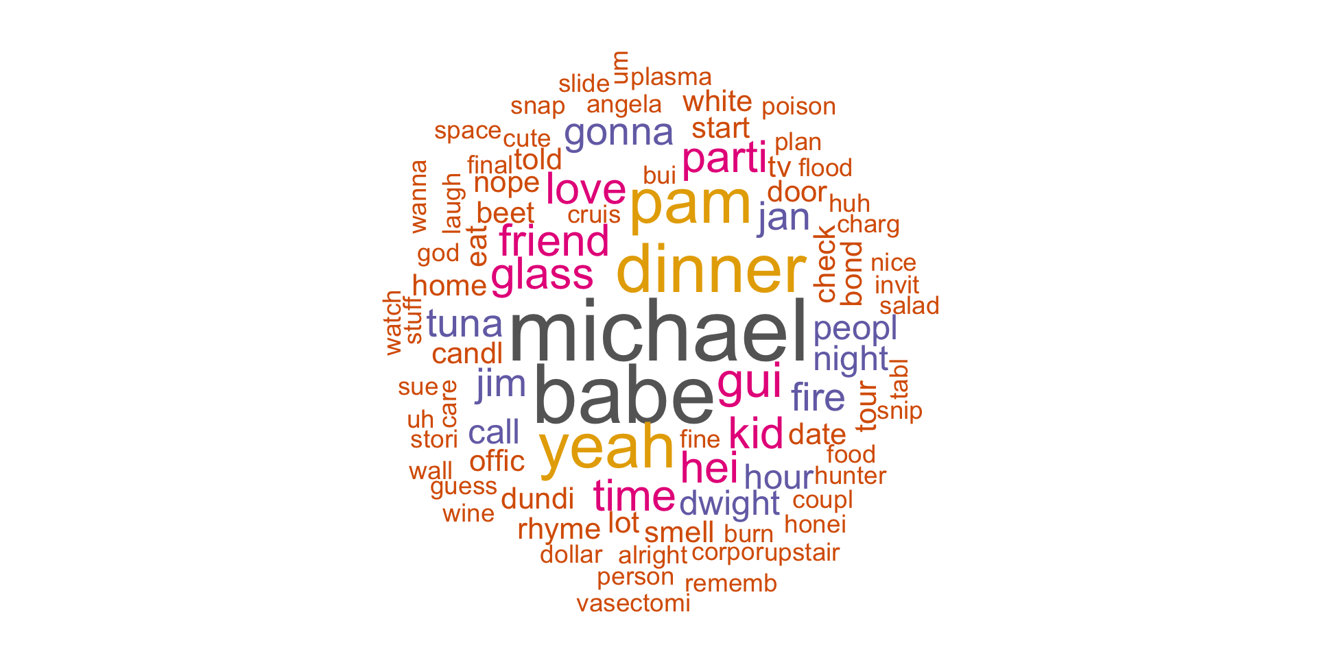
Bag of Words representation of text

• Most common way to store text data is with a document-term matrix (DTM):

	Word 1	Word 2	\(\dots\)	Word \(J\)
Document 1	\(w_{11}\)	\(w_{12}\)	\(\dots\)	\(w_{1J}\)
Document 2	\(w_{21}\)	\(w_{22}\)	\(\dots\)	\(w_{2J}\)
\(\dots\)	\(\dots\)	\(\dots\)	\(\dots\)	\(\dots\)
Document N	\(w_{N1}\)	\(w_{N2}\)	\(\dots\)	\(w_{NJ}\)

• \(w_{ij}\): count of word \(j\) in document \(i\), aka term frequencies

Two additional ways to reduce number of columns:

1. Stop words: remove extremely common words (e.g., of, the, a)

2. Stemming: Reduce all words to their “stem”

• For example: Reducing = reduc. Reduce = reduc. Reduces = reduc.

Tokenize text into long format

• Convert raw text into long, tidy table with one-token-per-document-per-row

  • A token equals a unit of text - typically a word

library(tidytext)
tidy_dinner_party_tokens <- dinner_party_table |>
  unnest_tokens(word, text)
head(tidy_dinner_party_tokens)

# A tibble: 6 × 3
  index character word      
  <int> <chr>     <chr>     
1 16791 Stanley   this      
2 16791 Stanley   is        
3 16791 Stanley   ridiculous
4 16792 Phyllis   do        
5 16792 Phyllis   you       
6 16792 Phyllis   have      

Easy to convert text into DTM format using tidytext package

Remove stop words

• Load stop_words from tidytext

data(stop_words)

tidy_dinner_party_tokens <- tidy_dinner_party_tokens |>
  filter(!(word %in% stop_words$word))

head(tidy_dinner_party_tokens)

# A tibble: 6 × 3
  index character word      
  <int> <chr>     <chr>     
1 16791 Stanley   ridiculous
2 16792 Phyllis   idea      
3 16792 Phyllis   time      
4 16793 Michael   likes     
5 16793 Michael   late      
6 16793 Michael   plans     

Apply stemming

• Can use SnowballC package to perform stemming

library(SnowballC)

tidy_dinner_party_tokens <- tidy_dinner_party_tokens |>
  mutate(stem = wordStem(word))

head(tidy_dinner_party_tokens)

# A tibble: 6 × 4
  index character word       stem   
  <int> <chr>     <chr>      <chr>  
1 16791 Stanley   ridiculous ridicul
2 16792 Phyllis   idea       idea   
3 16792 Phyllis   time       time   
4 16793 Michael   likes      like   
5 16793 Michael   late       late   
6 16793 Michael   plans      plan   

Create word cloud using term frequencies

Word Cloud: Displays all words mentioned across documents, where more common words are larger

• To do this, you must compute the total word counts:

\[w_{\cdot 1} = \sum_{i=1}^N w_{i1} \hspace{0.1in} \dots \hspace{0.1in} w_{\cdot J} = \sum_{i=1}^N w_{iJ}\]

• Then, the size of Word \(j\) is proportional to \(w_{\cdot j}\)

Create word clouds in R using wordcloud package

Takes in two main arguments to create word clouds:

1. words: vector of unique words

2. freq: vector of frequencies

Create word cloud using term frequencies

token_summary <- tidy_dinner_party_tokens |>
  group_by(stem) |>
  count() |>
  ungroup() 

library(wordcloud)
wordcloud(words = token_summary$stem, 
          freq = token_summary$n, 
          random.order = FALSE, 
          max.words = 100, 
          colors = brewer.pal(8, "Dark2"))

• Set random.order = FALSE to place biggest words in center

• Can customize to display limited # words (max.words)

• Other options as well like colors

Create word cloud using term frequencies

Comparison clouds

Imagine we have two different collections of documents, \(\mathcal{A}\) and \(\mathcal{B}\), that we wish to visually compare.

Imagine we create the word clouds for the two collections of documents. Then this means we constructed vectors of total words for each collection:

• \(\mathbf{w}^{\mathcal{A}} = (w_{\cdot 1}^{\mathcal{A}}, \dots, w_{\cdot J}^{\mathcal{A}})\)

• \(\mathbf{w}^{\mathcal{B}} = (w_{\cdot 1}^{\mathcal{B}}, \dots, w_{\cdot J}^{\mathcal{B}})\)

Consider the \(j\)th word, let’s pretend it’s “dinner”:

• If \(w_{\cdot j}^{\mathcal{A}}\) is large, then “dinner” is large in the word cloud for \(\mathcal{A}\).

• If \(w_{\cdot j}^{\mathcal{B}}\) is large, then “dinner” is large in the word cloud for \(\mathcal{B}\).

• But if both are large, this doesn’t tell us whether \(w_{\cdot j}^{\mathcal{A}}\) or \(w_{\cdot j}^{\mathcal{B}}\) is bigger.

Comparison clouds

This motivates the construction of comparison word clouds:

1. For word \(j\), compute \(\bar{w}_{\cdot j} = \text{average}(w_{\cdot j}^{\mathcal{A}}, w_{\cdot j}^{\mathcal{B}})\)

2. Compute \(w_{\cdot j}^{\mathcal{A}} - \bar{w}_{\cdot j}\) and \(w_{\cdot j}^{\mathcal{B}} - \bar{w}_{\cdot j}\)

3. If \(w_{\cdot j}^{\mathcal{A}} - \bar{w}_{\cdot j}\) is very positive, make it large for the \(\mathcal{A}\) word cloud. If \(w_{\cdot j}^{\mathcal{B}} - \bar{w}_{\cdot j}\) is very positive, make it large for the \(\mathcal{B}\) word cloud.

Comparison clouds

TF-IDF weighting

• We saw that michael was the largest word, but what if I’m interested in comparing text across characters (i.e., documents)?

• It’s arguably of more interest to understand which words are frequently used in one set of texts but not the other, i.e., which words are unique?

• Many text analytics methods will down-weight words that occur frequently across all documents

• Inverse document frequency (IDF): for word \(j\) we compute \(\text{idf}_j = \log \frac{N}{N_j}\)

  • where \(N\) is number of documents, \(N_j\) is number of documents with word \(j\)

• Compute TF-IDF \(= w_{ij} \times \text{idf}_j\)

TF-IDF example with characters

Compute and join TF-IDF using bind_tf_idf():

character_token_summary <- tidy_dinner_party_tokens |>
  group_by(character, stem) |> 
  count() |>
  ungroup() 

character_token_summary <- character_token_summary |>
  bind_tf_idf(stem, character, n) 
character_token_summary

# A tibble: 597 × 6
   character stem        n     tf   idf tf_idf
   <chr>     <chr>   <int>  <dbl> <dbl>  <dbl>
 1 All       cheer       1 1      2.77  2.77  
 2 Andy      anim        1 0.0476 2.77  0.132 
 3 Andy      bet         1 0.0476 2.08  0.0990
 4 Andy      capit       1 0.0476 2.77  0.132 
 5 Andy      dinner      1 0.0476 0.981 0.0467
 6 Andy      flower      2 0.0952 2.77  0.264 
 7 Andy      hei         1 0.0476 1.39  0.0660
 8 Andy      helena      1 0.0476 2.77  0.132 
 9 Andy      hump        2 0.0952 2.77  0.264 
10 Andy      michael     1 0.0476 0.981 0.0467
# ℹ 587 more rows

Top 10 words by TF-IDF for each character

character_token_summary |>
  filter(character %in% c("Michael", "Jan", "Jim", "Pam")) |>
  group_by(character) |>
  slice_max(tf_idf, n = 10, with_ties = FALSE) |>
  ungroup() |>
  mutate(stem = reorder_within(stem, tf_idf, character)) |>
  ggplot(aes(y = tf_idf, x = stem),
         fill = "darkblue", alpha = 0.5) +
  geom_col() +
  coord_flip() +
  scale_x_reordered() +
  facet_wrap(~ character, ncol = 2, scales = "free") +
  labs(y = "TF-IDF", x = NULL)

Top 10 words by TF-IDF for each character

Sentiment Analysis

• The visualizations so far only look at word frequency (possibly weighted with TF-IDF), but doesn’t tell you how words are used

• A common goal in text analysis is to try to understand the overall sentiment or “feeling” of text, i.e., sentiment analysis

• Typical approach:

  1. Find a sentiment dictionary (e.g., “positive” and “negative” words)

  2. Count the number of words belonging to each sentiment

  3. Using the counts, you can compute an “average sentiment” (e.g., positive counts - negative counts)

• This is called a dictionary-based approach

• The Bing dictionary (named after Bing Liu) provides 6,786 words that are either “positive” or “negative”

Character sentiment analysis

get_sentiments("bing")

# A tibble: 6,786 × 2
   word        sentiment
   <chr>       <chr>    
 1 2-faces     negative 
 2 abnormal    negative 
 3 abolish     negative 
 4 abominable  negative 
 5 abominably  negative 
 6 abominate   negative 
 7 abomination negative 
 8 abort       negative 
 9 aborted     negative 
10 aborts      negative 
# ℹ 6,776 more rows

Character sentiment analysis

Join sentiment to token table (without stemming)

tidy_all_tokens <- dinner_party_table |>
  unnest_tokens(word, text)

tidy_sentiment_tokens <- tidy_all_tokens |>
  inner_join(get_sentiments("bing")) 

head(tidy_sentiment_tokens)

# A tibble: 6 × 4
  index character word       sentiment
  <int> <chr>     <chr>      <chr>    
1 16791 Stanley   ridiculous negative 
2 16793 Michael   likes      positive 
3 16793 Michael   work       positive 
4 16795 Michael   enough     positive 
5 16795 Michael   enough     positive 
6 16795 Michael   mad        negative 

Character sentiment analysis

tidy_sentiment_tokens |>
  group_by(character, sentiment) |>
  summarize(n_words = n()) |>
  ungroup() |>
  group_by(character) |>
  mutate(total_assigned_words = sum(n_words)) |>
  ungroup() |>
  mutate(character = fct_reorder(character, total_assigned_words)) |>
  ggplot(aes(x = character, y = n_words, fill = sentiment)) + 
  geom_bar(stat = "identity") +
  coord_flip() +
  scale_fill_manual(values = c("red", "blue")) +
  theme_bw() +
  theme(legend.position = "bottom")

Character sentiment analysis

Other functions of text

• We’ve just focused on word counts - but there are many functions of text

• For example: number of unique words is often used to measure vocabulary

Recap and next steps

• Most common representation: Bag of words and term frequencies (possibly weighted by TF-IDF)

• Word clouds are the most common way to visualize the most frequent words in a set of documents

• TF-IDF weighting allows you to detect words that are uniquely used in certain documents

• Can also measure the “sentiment” of text with sentiment-based dictionaries

• Infographic is due Friday night!

• Text Mining With R, Supervised Machine Learning for Text Analysis in R