INSTRUCTOR SOLUTIONS: Introduction to regularized adjusted plus-minus (RAPM)

An introduction to ridge regression in the context of estimating basketball player effects.

Intro and Data

The purpose of this module is to walk through the basics of building a regularized adjusted plus-minus (RAPM) model to estimate the impact of basketball players when they are on the court, while adjusting for the quality of their teammates and opponents.

We’ll use NBA data available on the SCORE Network Data repository, that was already constructed for the purpose of building and comparing different approaches for estimating player effects. The data were gathered using the hoopR package, you can find the script for initializing the data on GitHub.

The following code chunk reads in a dataset that is in a wide form (discussed in detail below) with indicator columns for every player that was observed during the 2022-23 regular season:

# Need to have the tidyverse installed prior to starting!
library(tidyverse)
nba_rapm_data <- read_csv("https://data.scorenetwork.org/data/nba_2223_season_rapm_data.csv.gz")

In this dataset, we have 32,358 unique shifts/stints with 539 players represented by the indicator variables (+1 if on court for home team, -1 if on court for away team, and 0 if not on court). Additional context is captured by the following variables:

Variable	Description
game_id	Unique game ID
stint_id	Unique identifier within a game for a stint for particular combination of home and away lineup (in appearance of order, where 1 is the first stint in the game)
n_pos	Number of possessions (combined for both home and away) during the observed stint
home_points	Number of points scored by the home team during the stint
away_points	Number of points scored by the away team during the stint
minutes	Length of the stint in terms of minutes played
margin	Common response for RAPM models defined as: (home_points - away_points) / n_pos * 100

Since the above dataset does not include player names, only unique identifiers, we will also load in a table that includes player names to join over with the eventual results of the analysis. You can use the code chunk below to read in this table from the SCORE Network Data repository:

nba_player_table <- read_csv("https://data.scorenetwork.org/data/nba_2223_player_table.csv")

Rows: 539 Columns: 2
── Column specification ────────────────────────────────────────────────────────
Delimiter: ","
chr (1): player_name
dbl (1): player_id

ℹ Use `spec()` to retrieve the full column specification for this data.
ℹ Specify the column types or set `show_col_types = FALSE` to quiet this message.

nba_player_table

# A tibble: 539 × 2
   player_id player_name             
       <dbl> <chr>                   
 1   1630173 Precious Achiuwa        
 2    203500 Steven Adams            
 3   1628389 Bam Adebayo             
 4   1630534 Ochai Agbaji            
 5   1630583 Santi Aldama            
 6   1629638 Nickeil Alexander-Walker
 7   1628960 Grayson Allen           
 8   1628386 Jarrett Allen           
 9   1630631 Jose Alvarado           
10    203937 Kyle Anderson           
# ℹ 529 more rows

Background Information

Measuring a player’s effect on game outcomes is one of the most fundamental tasks in sports analytics. But this is not a simple thing to do, and varies greatly between sports! In sports like basketball and hockey, a popular starting point for measuring a player’s impact is Plus-Minus which is defind as:

Plus-Minus = points scored by team when player is on court - points scored by opposing team when player is on court

You can find leaderboards for this statistic on the NBA stats website.

Thought Exercise

QUESTION: What do you think are potential limitations with the above Plus-Minus statistic?

ANSWER: The naive version of Plus-Minus ignores the influence of a player’s teammates and the opponents they faced during their time on the court. If a “bad” player shares court with a “good” player, they may have a strong positive Plus-Minus since their “good” teammate can offset the “bad” player (and vice versa). Likewise, if a “good” player has a more difficult schedule against stronger opponents then it can potentially hurt their Plus-Minus (with the opposite true against an easier schedule of weaker opponents).

We’ll now walk through how to improve on Plus-Minus with regression-based approaches using the NBA data loaded in the beginning of the module.

Learn By Doing

Adjusted Plus-Minus (APM)

Introduced by Rosenbaum (2004), adjusted Plus-Minus (APM) is a regression-based approach to estimate a player’s impact on game outcomes while accounting for their teammates and opponents. How does this work? APM is a regression model where the predictors are indicator variable for every player denoting if they are on the court. The response variable is some type of outcome observed as the possession or shift-level (explained below). To be more explicit:

• There are 10 players on the court at a time during a basketball game, 5 on side and 5 on the other.

• A basketball game has \(T\) shifts (or stints) that are periods of time without substitutions (i.e., there are no changes to who are playing on the court).

• We will consider each 10-person shift \(t = 1,\dots,T\) to be a single observation.

• The reponse variable is some type of game outcome measure, such as the score differential during shift \(t\) from the view of the home team (i.e., home team score - away team score).

• The predictor variables represented in the \(T \times p\) design matrix \(X\) are columns for each of the \(p\) players in the league, such that:

  • \(X_{tj} = 1\) if player \(j\) is on the court for the home team during shift \(t\)
  • \(X_{tj} = -1\) if player \(j\) is on the court for the away team during shift \(t\)
  • \(X_{tj} = 0\) if player \(j\) is not on the court during shift \(t\)

Note

There are a number of different ways to set-up the APM design matrix \(X\), but we will only consider this design based on home and away team status in this module.

As discussed at the beginning of this module, the nba_rapm_data you loaded contains these player indicator variables. The code chunk below prints the first so many rows of this dataset:

nba_rapm_data

# A tibble: 32,358 × 546
   game_id    stint_id n_pos home_points away_points minutes margin `201939`
   <chr>         <dbl> <dbl>       <dbl>       <dbl>   <dbl>  <dbl>    <dbl>
 1 0022200002        1    14           5           2   2.7     21.4        1
 2 0022200002        2     9           6           2   1.67    44.4        1
 3 0022200002        3     5           0           3   0.480  -60          1
 4 0022200002        4     5           5           1   0.78    80          1
 5 0022200002        5     9           3           6   1.52   -33.3        1
 6 0022200002        6     8           0           6   1.45   -75          1
 7 0022200002        7     5           0           0   0.800    0          0
 8 0022200002        8     5           1           0   0.9     20          0
 9 0022200002        9     3           2           0   0.97    66.7        0
10 0022200002       10     7           2           2   1.66     0          1
# ℹ 32,348 more rows
# ℹ 538 more variables: `202691` <dbl>, `203110` <dbl>, `203952` <dbl>,
#   `1626172` <dbl>, `1629673` <dbl>, `203210` <dbl>, `1630164` <dbl>,
#   `1630228` <dbl>, `1628978` <dbl>, `1630541` <dbl>, `1631157` <dbl>,
#   `201143` <dbl>, `203935` <dbl>, `1627759` <dbl>, `1628369` <dbl>,
#   `1628401` <dbl>, `203943` <dbl>, `1629684` <dbl>, `1627763` <dbl>,
#   `201933` <dbl>, `1630573` <dbl>, `101108` <dbl>, `1626164` <dbl>, …

The Rosenbaum (2004) implementation of APM relies on weighted least squares, where you solve for the \(p\)-dimensional vector of player coefficients \(\boldsymbol{\beta}\) using a modified version of the traditional least squares model:

\[ \hat{\boldsymbol{\beta}} = \underset{\boldsymbol{\beta} \in \mathbb{R}^p}{\text{arg min}} \sum_{t = 1}^T n_t (y_t - X_t \boldsymbol{\beta})^2 \] * \(y_t\) is the response variable during shift \(t\), * \(X_t\) is the row of the design matrix for shift \(t\), and * \(n_t\) is the number possessions during shift \(t\).

Thought Exercise

QUESTION: What do you think is the motivation behind using weighted least squares rather than ordinary least squares without weights? Think about the choice of using the number of possessions as the weights.

ANSWER: Since a shift of time can vary in length, the idea behind using the number of possessions as weights is to place more importance on observations that effectively capture more periods of game play. Observed shifts with more possessions should be more informative about player performance than shifts with fewer possessions.

We’ll now work through fitting and intepreting the APM model in the context of NBA 2022-23 regular season data.

First, compute the score differential as score_diff = home_points - away_points using mutate(). Append this new column to the nba_rapm_data dataset.

nba_rapm_data <- nba_rapm_data |>
  mutate(score_diff = home_points - away_points)

Next, create a new dataset named nba_apm_model_data that contains only the response score_diff and the player columns:

nba_apm_model_data <- nba_rapm_data |>
  dplyr::select(-c(game_id, stint_id, n_pos, home_points, away_points, minutes,
                   margin))

Next, fit the model using the code below:

rosenbaum_model <- lm(score_diff ~ 0 + ., data = nba_apm_model_data,
                      weights = nba_rapm_data$n_pos)

Note

Compared to fitting a linear regression model in R using the lm() with a small number of predictors, this model has the following aspects:

• The intercept term is not included by specifying 0 at the beginning of the formula,

• Using + . in the formula tells lm() to use every column in the data as predictors,

• weights = nba_rapm_data$n_pos ensures that we are using weighted least squares with the n_pos column (number of possessions during the shift) as the weights.

Thought Exercise

QUESTION: Why is it appropriate to remove the intercept term in the above regression model?

ANSWER: We need to remove the intercept term in the APM because it is impossible for every column of \(X\) to be 0, i.e., we will always observe 10 columns to have non-zero values in every single row of the dataset. This means the intercept term is nonsensical and should be removed from model fitting.

We’re not going to view the summary of this model since it is a bit of a mess (there are many player variables!). Instead, we’ll take advantage of the broom package to view the coefficients. The code chunk below demonstrates how to use the broom package to tidy up the output so that one row of the rosenbaum_coef table corresponds to a single player coefficient with information you would observe from the summary() output such as the coefficient estimate (estimate), standard error (std.error), \(t\)-statistic (statistic), \(p\)-value (p.value):

library(broom)
rosenbaum_coef <- tidy(rosenbaum_model)
rosenbaum_coef

# A tibble: 539 × 5
   term      estimate std.error statistic p.value
   <chr>        <dbl>     <dbl>     <dbl>   <dbl>
 1 `201939`   -0.303       1.58   -0.192    0.848
 2 `202691`   -1.01        1.58   -0.641    0.521
 3 `203110`    0.214       1.58    0.135    0.892
 4 `203952`    0.0336      1.58    0.0213   0.983
 5 `1626172`  -0.417       1.58   -0.265    0.791
 6 `1629673`  -1.36        1.57   -0.866    0.386
 7 `203210`   -0.971       1.58   -0.613    0.540
 8 `1630164`  -1.02        1.59   -0.640    0.522
 9 `1630228`  -0.663       1.58   -0.421    0.674
10 `1628978`  -0.565       1.57   -0.359    0.720
# ℹ 529 more rows

In this current form, we have no idea which player is which since the term column contains the unique ID for each player. However, we can take advantage of the previously loaded nba_player_table (which has the same number of rows as rosenbaum_coef) to join over the player names to the rosenbaum_coef table.

We first need to modify the term column by removing the back-tick symbols and then convert the IDs to numeric values before joining over the player names. The code chunk below performs these steps, using the left_join() function by matching the two tables on the term and player_id columns:

rosenbaum_coef <- rosenbaum_coef |>
  # First convert the term column to numeric:
  mutate(term = as.numeric(str_remove_all(term, "`"))) |>
  # Now join the player names:
  left_join(nba_player_table, by = c("term" = "player_id"))
rosenbaum_coef

# A tibble: 539 × 6
      term estimate std.error statistic p.value player_name     
     <dbl>    <dbl>     <dbl>     <dbl>   <dbl> <chr>           
 1  201939  -0.303       1.58   -0.192    0.848 Stephen Curry   
 2  202691  -1.01        1.58   -0.641    0.521 Klay Thompson   
 3  203110   0.214       1.58    0.135    0.892 Draymond Green  
 4  203952   0.0336      1.58    0.0213   0.983 Andrew Wiggins  
 5 1626172  -0.417       1.58   -0.265    0.791 Kevon Looney    
 6 1629673  -1.36        1.57   -0.866    0.386 Jordan Poole    
 7  203210  -0.971       1.58   -0.613    0.540 JaMychal Green  
 8 1630164  -1.02        1.59   -0.640    0.522 James Wiseman   
 9 1630228  -0.663       1.58   -0.421    0.674 Jonathan Kuminga
10 1628978  -0.565       1.57   -0.359    0.720 Donte DiVincenzo
# ℹ 529 more rows

Now with the player names joined, let’s examine which players are the top 10 and bottom 10 in terms of their reported APM coefficients. You could easily view the top 10 players with the slice_max() function as demonstrated in the code chunk below:

rosenbaum_coef |>
  slice_max(estimate, n = 10)

# A tibble: 10 × 6
      term estimate std.error statistic p.value player_name     
     <dbl>    <dbl>     <dbl>     <dbl>   <dbl> <chr>           
 1 1629735     5.72      2.66     2.15   0.0314 Chris Silva     
 2 1631495     4.82      3.41     1.41   0.157  Donovan Williams
 3 1630648     4.04      3.26     1.24   0.215  Jordan Schakel  
 4 1629126     2.71      2.83     0.960  0.337  Deonte Burton   
 5 1630600     2.71      1.86     1.46   0.145  Isaiah Mobley   
 6 1629714     2.45      1.94     1.27   0.205  Jarrell Brantley
 7 1641645     2.03      1.82     1.11   0.265  Xavier Cooks    
 8 1630649     1.92      4.61     0.417  0.677  Stanley Umude   
 9 1630644     1.40      2.11     0.664  0.507  Mac McClung     
10 1628371     1.33      1.65     0.810  0.418  Jonathan Isaac  

And similarly use slice_min() to display the bottom 10:

rosenbaum_coef |>
  slice_min(estimate, n = 10)

# A tibble: 10 × 6
      term estimate std.error statistic p.value player_name    
     <dbl>    <dbl>     <dbl>     <dbl>   <dbl> <chr>          
 1 1631211    -8.43      2.65     -3.19 0.00144 Trevor Keels   
 2 1630241    -5.95      1.91     -3.12 0.00181 Sam Merrill    
 3 1628435    -5.26      2.24     -2.35 0.0190  Chance Comanche
 4 1630225    -3.93      1.92     -2.04 0.0410  Isaiah Todd    
 5 1630206    -3.80      2.08     -1.83 0.0672  Jay Scrubb     
 6 1628382    -3.58      1.73     -2.07 0.0381  Justin Jackson 
 7 1631157    -3.29      1.75     -1.88 0.0607  Ryan Rollins   
 8 1631311    -3.02      2.31     -1.31 0.191   Lester Quinones
 9 1631320    -3.00      2.67     -1.12 0.261   Chima Moneke   
10 1630643    -2.90      1.84     -1.58 0.115   Jay Huff       

These look like pretty extreme values, with the most extreme values observed by players that have limited playing time (upon searching their stats online). Before we think about how to address these issues, let’s look at what happens if we make a slight tweak to our model by using the margin variable as the response instead which is defined as:

margin = (home_points - away_points) / n_pos * 100

This response is often preferred in the basketball analytics community, as it places the response on a scale of points per 100 possessions (which is comparable to the number of possessions in each basketball game).

Active Exercise

QUESTION:

Repeat the steps from above, but fit a new regression model using the margin variable in the original data nba_rapm_data as the response instead of score_diff. Do NOT include any weights since the number of possessions is already accounted for in margin. Report the top 10 players based on this new APM model with margin. How do the rankings and estimates compare to the Rosenbaum APM model from above?

ANSWER:

# Now for ease, create a dataset that only has the response and player columns:
nba_margin_apm_model_data <- nba_rapm_data |>
  dplyr::select(-c(game_id, stint_id, n_pos, home_points, away_points, minutes,
                   score_diff))

# Fit the model (notice we do not include an intercept term)
rosenbaum_margin_model <- lm(margin ~ 0 + ., data = nba_margin_apm_model_data)

# Get the coefficients and join player names:
rosenbaum_margin_coef <- tidy(rosenbaum_margin_model) |>
  # First convert the term column to numeric:
  mutate(term = as.numeric(str_remove_all(term, "`"))) |>
  # Now join the player names:
  left_join(nba_player_table, by = c("term" = "player_id"))

# View top 10:
rosenbaum_margin_coef |>
  slice_max(estimate, n = 10)

# A tibble: 10 × 6
      term estimate std.error statistic p.value player_name     
     <dbl>    <dbl>     <dbl>     <dbl>   <dbl> <chr>           
 1 1630649     75.4      52.0     1.45    0.147 Stanley Umude   
 2 1630648     60.6      53.1     1.14    0.253 Jordan Schakel  
 3 1628993     49.1      31.5     1.56    0.119 Alize Johnson   
 4 1630250     49.1      36.4     1.35    0.177 Marko Simonovic 
 5 1629126     45.4      51.2     0.888   0.375 Deonte Burton   
 6 1631495     45.1      60.3     0.748   0.455 Donovan Williams
 7 1630600     40.1      31.7     1.27    0.205 Isaiah Mobley   
 8  203999     36.2      27.5     1.32    0.187 Nikola Jokic    
 9 1628973     35.6      27.4     1.30    0.193 Jalen Brunson   
10 1631112     35.1      30.7     1.14    0.253 Kendall Brown   

We start to see names that make sense, like Nikola Jokic who was one of the best players in the NBA during the 2022-23 season. We also notice the difference in magnitude now for the coefficient estimates compared to the previous score differential model. This is because the response is on the scale of points per 100 possessions.

Active Exercise

QUESTION: Using the results of your margin-based model. Create a visualization displaying the distribution of the player coefficients. Describe what you observe about this distribution.

ANSWER:

rosenbaum_margin_coef |>
  ggplot(aes(x = estimate)) +
  geom_histogram() +
  labs(x = "APM estimate", y = "Count") +
  theme_bw()

`stat_bin()` using `bins = 30`. Pick better value with `binwidth`.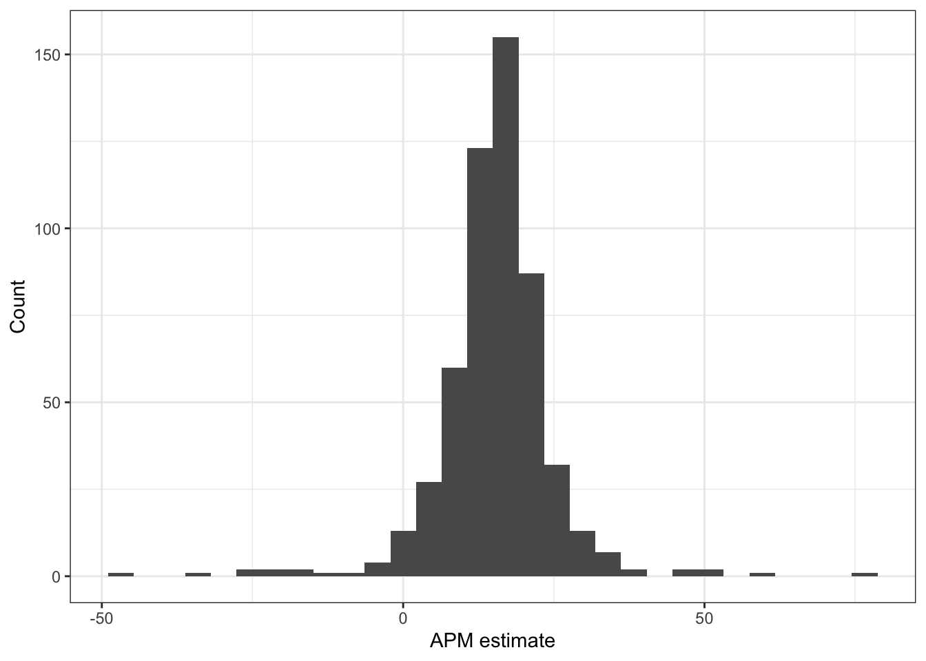

We can see that the coefficient distribution is roughly normal looking! We observe that most players display coefficients within a reasonable range but we do see some extreme looking values on the tail ends. This motivates the role of thinking about a group-level distribution for which player coefficients may come from.

Thought Exercise

QUESTION: What do you think are potential issues and concerns with the APM model?

ANSWER: There are number of different concerns regarding the APM model:

• High-dimensional problem: There are hundreds of player coefficients to estimate in the model. This is a high-dimensional regression problem, thus meaning that we need sufficient amount of data to estimate appropriately.

• Multicollinearity: Players are often substituted in and out simultaneously, or for one another - without adjustments. This will lead to collinearity between player columns, which can result in larger variance for the player coefficients, as well as decreases the precision of estimates. The challenge of multicollinearity makes it more difficult to parse between which players deserve more credit.

• Limited playing time: For players with limited playing time, we may observe unstable and extreme coefficient values. There are different ways to address this (such as the way we’ll handle it in RAPM), but one option in APM is to replace all players with limited playing time as single column, i.e., replacement-level player.

Regularized Adjusted Plus-Minus (RAPM)

Next, we’ll address some of the common issues facing APM models using Regularized Adjusted Plus-Minus (RAPM). The first public instance of RAPM for basketball was by Joe Sill (2010) in an award winning research paper at a sports analytics conference. This version of RAPM relies on ridge regression to apply a penalty term for shrinking player coefficients. More specifically, we can update the previous formula for estimating player coefficients as follows:

\[ \hat{\boldsymbol{\beta}}^{ridge} = \underset{\boldsymbol{\beta} \in \mathbb{R}^p}{\text{arg min}} \sum_{t = 1}^T (y_t - X_t \boldsymbol{\beta})^2 + \lambda \sum_{j = 1}^p \beta_p^2 \]

This objective for the ridge regression coefficients is effectively the combination of the loss (the traditional least squares objective) and newly included penalty term (the sum of the squared coefficient values). The ridge regression coefficients are solved for while balancing these two terms simultaneously, with the amount penalization controlled by \(\lambda\). We can consider \(\lambda\) to be a tuning parameter that controls the strength of the penalty term, and we will want to choose the \(\lambda\) based on out-of-sample performance.

Thought Exercise

QUESTION: What happens to the coefficients if \(\lambda = 0\)? What happens to the coefficients as \(\lambda \rightarrow + \infty\)?

ANSWER:

• If \(\lambda = 0\): we just observe the same coefficients from fitting ordinary least squares, with no penalty term included.

• As \(\lambda \rightarrow + \infty\): the coefficients shrink towards 0, but never actually equal zero.

Challenging Exercise

QUESTION: Ignoring the context of RAPM models, suppose you regress a response variable \(Y\) on two variables \(X_1\) and \(X_2\) where \(X_1 = X_2\). What is the solution to ridge regression in this case? Do you think this behavior is ideal in the context of estimating player effects in the presence of collinearity?

ANSWER:

If we plug in the two variables in the ridge regression objective function from above, and use the Euclidean norm notation of the squared terms, then the loss and penalty terms become:

\[ || Y - X_1 \beta_1 - X_2 \beta_2 ||_2^2 + \lambda \beta_1^2 + \lambda \beta_2^2 \] And since \(X_1 = X_2\), we can set \(X = X_1 = X_2\) so that this becomes:

\[ || Y - X (\beta_1 + \beta_2) ||_2^2 + \lambda (\beta_1^2 + \beta_2^2) \] Due to the quadratic constraint from \(\lambda (\beta_1^2 + \beta_2^2)\), the unique solution to this objective is to set \(\beta_1 = \beta_2\)! Thus when two variables are perfectly equal to each other, they will receive equal coefficients in ridge regression.

In the context of modeling player effects in sports, this can be useful because it is signaling that we do not know how to distinguish two players from each other if we only ever observed them together - so the resulting coefficients will treat them as equal. However, the downside is that we likely have prior knowledge about the players and could benefit from including that somehow. Incorporating priors into RAPM models via Bayesian regression is beyond the scope of this module.

We’ll now walk through how to fit a RAPM model using ridge regression. The most popular implementation of fitting ridge regression (and other common penalized regression models) in R is with the glmnet package.

First, grab only the player columns (i.e. the indicator variables in the original data), then convert to a matrix using as.matrix(), and store this as a new object named player_matrix.

player_matrix <- nba_margin_apm_model_data |>
  dplyr::select(-margin) |>
  as.matrix()

Next, the code chunk below performs 10 fold cross-validation to fit a ridge regression model using glmnet. The function cv.glmnet is used to perform the 10 fold cross-validation, evaluating the out-of-sample performance for a grid of \(\lambda\) values. Fill in the missing code below using the above player_matrix as the predictors with the margin variable as the response:

library(glmnet)

Loading required package: Matrix

Warning: package 'Matrix' was built under R version 4.2.3

Attaching package: 'Matrix'

The following objects are masked from 'package:tidyr':

    expand, pack, unpack

Loaded glmnet 4.1-8

# View help for function with:
# help(cv.glmnet)

# ridge with 10 fold cv, no intercept and no standardization
fit_ridge_cv <- cv.glmnet(x = player_matrix,
                          y = nba_margin_apm_model_data$margin,
                          alpha = 0,
                          intercept = FALSE,
                          standardize = FALSE)

The following plot prints out the penalty selection for this model, with the choices for \(\lambda\) displayed along the x-axis and the 10 fold cross-validation mean squared error displayed along the y-axis. The red points denote the average error across the 10 folds, with gray standard error intervals.

plot(fit_ridge_cv)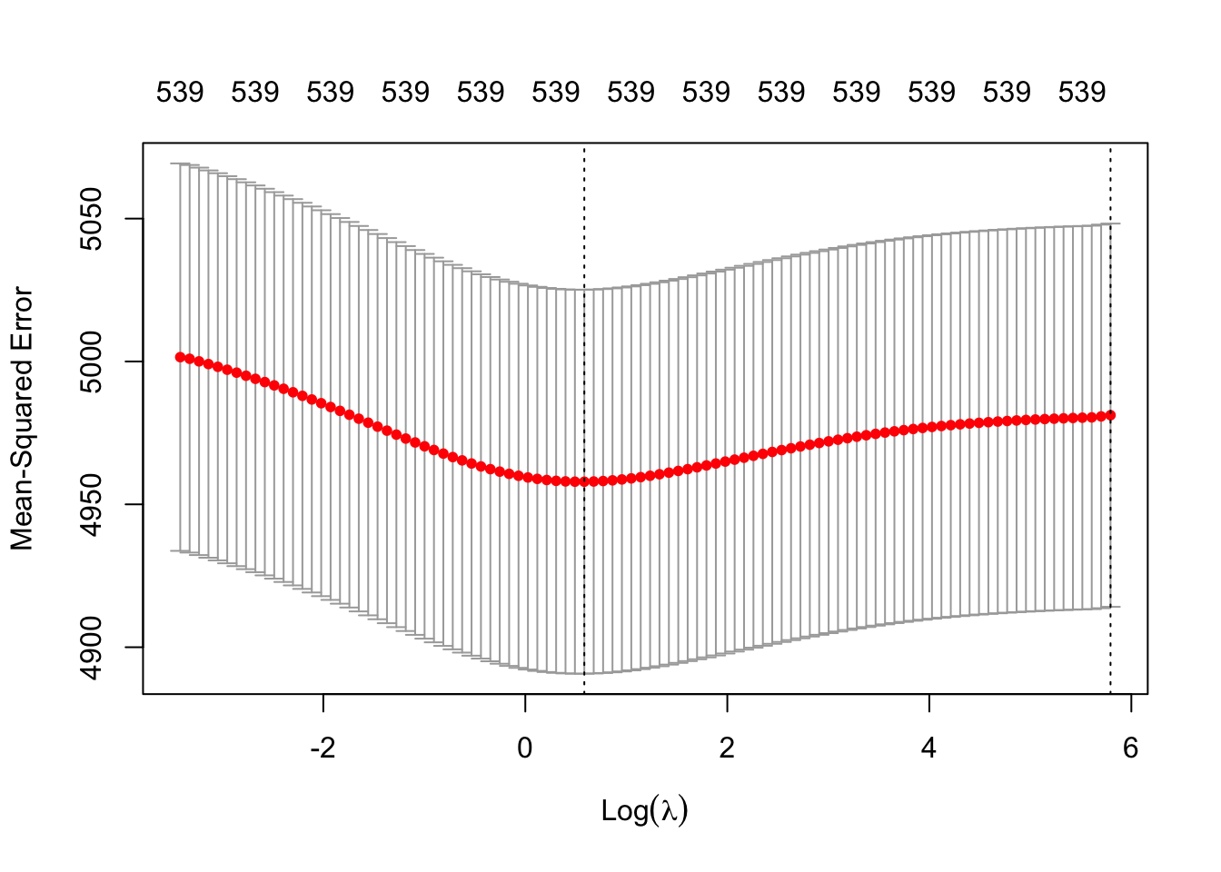

The first vertical dashed line corresponds to the choice of \(\lambda\) with the smallest average error across the 10 folds. The far right dashed line indicates the largest \(\lambda\) that is within one standard error of the minimum error \(\lambda\). Using this \(\lambda\) value is often referred to as the “one-standard error rule” as it implies picking a more “conservative” model with more penalized coefficients. In this case, we will prefer to choose the minimum error \(\lambda\) indicated with the first vertical dashed line.

Thought Exercise

QUESTION: What do you think the implication is that all of the red points are within the gray standard error intervals for all possible \(\lambda\) values?

ANSWER: This signals that in terms of out-of-sample performance, all of the choices of \(\lambda\) are fairly similar, indicating large uncertainty about the model’s predictive performance. However, we are primarily interested in estimating player effects with RAPM and not necessarily concerned with the model’s predictive performance.

We can easily plot the path of the ridge regression shrinkage, to see how the coefficients are pulled towards 0 as the penalty increases. The following code chunk shows this full path:

plot(fit_ridge_cv$glmnet.fit, xvar = "lambda")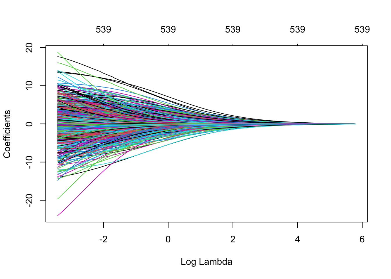

Similar to the APM model analyis, we can again use the the broom package to make a tidy table of the coefficients for each player:

tidy_ridge_coef <- tidy(fit_ridge_cv$glmnet.fit)
tidy_ridge_coef

# A tibble: 53,900 × 5
   term    step estimate lambda dev.ratio
   <chr>  <dbl>    <dbl>  <dbl>     <dbl>
 1 201939     1 2.77e-39   328.  1.45e-39
 2 201939     2 6.41e- 4   299.  3.30e- 4
 3 201939     3 7.23e- 4   273.  3.59e- 4
 4 201939     4 7.91e- 4   248.  3.93e- 4
 5 201939     5 8.69e- 4   226.  4.30e- 4
 6 201939     6 9.54e- 4   206.  4.70e- 4
 7 201939     7 1.05e- 3   188.  5.14e- 4
 8 201939     8 1.15e- 3   171.  5.62e- 4
 9 201939     9 1.27e- 3   156.  6.14e- 4
10 201939    10 1.39e- 3   142.  6.70e- 4
# ℹ 53,890 more rows

If you look closely, this returns 100 rows for each player in the data - because it is returning the coefficient for each player at each value of the lambda penalty. We can filter to the values for the optimal choice of lambda based on the cross-validation results, and then join our player names as before:

rapm_ridge_coef <- tidy_ridge_coef |>
  filter(lambda == fit_ridge_cv$lambda.min) |>
  # Convert term to numeric:
  mutate(term = as.numeric(term)) |>
  # Now join the player names:
  left_join(nba_player_table, by = c("term" = "player_id"))

Active Exercise

QUESTION:

Now, display the top 10 players based on coefficient estimates. What do you think of list in comparison to the APM results. Does this list pass the “eye test”? (Search who won the NBA MVP in 2023.)

ANSWER:

rapm_ridge_coef |>
  slice_max(estimate, n = 10) |>
  dplyr::select(term, player_name, estimate)

# A tibble: 10 × 3
      term player_name     estimate
     <dbl> <chr>              <dbl>
 1  203954 Joel Embiid         5.37
 2  203999 Nikola Jokic        4.59
 3 1629027 Trae Young          4.28
 4 1627783 Pascal Siakam       4.02
 5 1628973 Jalen Brunson       3.64
 6  201567 Kevin Love          3.59
 7  203110 Draymond Green      3.56
 8  201572 Brook Lopez         3.28
 9  203076 Anthony Davis       3.24
10 1629627 Zion Williamson     3.22

Considering Embiid won the MVP last season, this list definitely passes the eye test (it’s honestly amazing how well this works for basketball data). For context, let’s view the bottom 10:

rapm_ridge_coef |>
  slice_min(estimate, n = 10) |>
  dplyr::select(term, player_name, estimate)

# A tibble: 10 × 3
      term player_name        estimate
     <dbl> <chr>                 <dbl>
 1 1630558 Davion Mitchell       -3.92
 2 1630170 Devin Vassell         -3.86
 3 1629670 Jordan Nwora          -3.11
 4 1630598 Aaron Wiggins         -3.06
 5  203210 JaMychal Green        -3.02
 6 1630528 Josh Christopher      -2.95
 7 1630586 Usman Garuba          -2.93
 8 1631128 Christian Braun       -2.86
 9  203115 Will Barton           -2.59
10 1630197 Aleksej Pokusevski    -2.45

Active Exercise

QUESTION: Similar to before, create a visualization displaying the distribution of the player coefficients from this ridge regression RAPM. Describe what you observe about this distribution and how it compares to the APM coefficient distribution.

ANSWER:

rapm_ridge_coef |>
  ggplot(aes(x = estimate)) +
  geom_histogram() +
  labs(x = "RAPM estimate", y = "Count") +
  theme_bw()

`stat_bin()` using `bins = 30`. Pick better value with `binwidth`.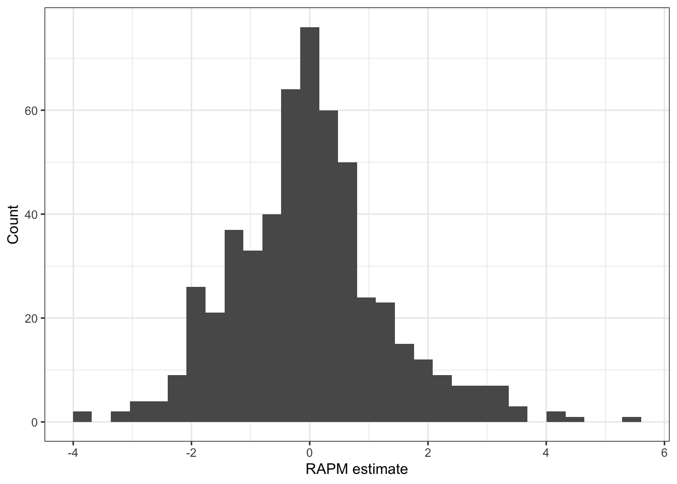

We can see that the RAPM coefficients also appear to roughly follow a Normal-like distribution, but we no longer observe extreme tails. Additionally, we can see that the center for this distribution is approximately 0! The use of penalization has shrunk players towards 0, serving as the average baseline for players. This leads to a nice interpretation that coefficients above 0 are above average in performance, while below 0 are below average in performance.

Discussion

You have now learned the basics behind RAPM models in the context of studying NBA player effects. We demonstrated how RAPM improves upon the simpler APM model, but there are still further questions and extensions to explore:

• Evaluating and tuning RAPM models: We only considered tuning the \(\lambda\) penalty via the default cross-validation in glmnet that relies on the observation-level response variable which in this case was the margin during an individual shift. However, the ultimate goal of the RAPM player coefficients could be for predicting game outcomes between two teams. One could tune the choice of \(\lambda\) based on predicting the game outcomes as a difference between the sum of the home and away team ratings.

• Alternative choices for design matrix: There is flexibility in the design matrix for RAPM models. We only considered the home/away version of the matrix in this module, but we could specify an alternative set-up so that offense and defense effects are estimated separately. This type of approach would split the shifts into possessions where one team is on offense and the other is on defense. Each player has two columns - one indicator column if they were on offense during the possession and another indicator if there were on defense. This provides two measures of player performance but can be more difficult to fit appropriately since this is doubling the dimensionality of the problem.

• Prior information: This module only considered estimating player performance based on the observed appearances in games. But what if we have prior knowledge to tease apart players who often appear on the court together? We could account for priors via a Bayesian version of the RAPM model. Details of this type of approach will be left to be covered in a future module!